 Learn About Structures
External reactions are usually the easiest forces to use as redundant forces for a force method analysis. But what could we do if our structure is internally indeterminate, but externally determinate (i.e. if we remove a reaction, then our structure will be unstable)? In this case, we can use an internal force, such as an axial force, or internal moment to act as the redundant force. Recall that the redundant force is the force that we remove to get the determinate primary structure as discussed in the previous section. Another situation when an internal redundant may be useful is when the use of an internal redundant results in a primary structure that is particularly easy to analyse.
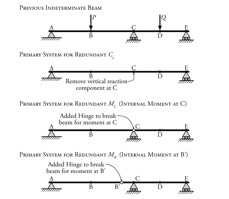
For the single degree indeterminate beam that we studied in the previous section (from Figure 8.1), if we consider the use of internal redundants then there are an infinite number of different redundants that we could choose. Three of these are shown in Figure 8.8. The top of the figure shows the previously studied single degree indeterminate beam. The second diagram from the top shows the primary system (the system with the redundant reaction removed) if the chosen redundant force is the reaction at point C ($C_y$). This is the example that was studied in Section 8.2. The third shows a potential internal redundant force, the internal moment at point C ($M_C$). For an external reaction redundant, we simply remove the reaction, but for an internal redundant, we must release whatever effect or continuity that redundant force is associated with. In this case, the internal moment at point C is associated with the transfer of moment through the beam from the left side of point C to the right. To remove the effect of this redundant, we must add a hinge at point C, effectively 'breaking' the beam's ability to resist moment at point C. Before adding the hinge, the beam could transfer moment at point C. The consequence is that the slope of the beam at point C must be continuous on either side of point C. The effect of adding the hinge (and breaking the moment transfer) is to have a 'kink' in the deflected shape of the beam, which will be shown later. The bottom diagram in the figure shows another potential position for an internal moment redundant in the beam: to the left of point C, at newly-identified point B'. There are an infinite number of potential locations for an internal moment redundant in this beam, because the internal redundant may be located anywhere along the length of the beam. Any position for the added hinge in this beam will make the system determinate and, therefore, appropriate for use as a primary system for the force method analysis; however, it is clear that some locations are more convenient for analysis than others. Locating the internal moment redundant at point C effectively converts the indeterminate beam into two adjacent simply-supported beams, which would be quite simple to analyse.
For internal redundant forces, the same rule applies that was previously used for the external reaction redundant forces: the removal of the restraint or continuity that is associated with an internal redundant force must not cause the structure to become unstable.
Beams and Frames
For a beam or frame element, the most common type of internal redundant for a force method analysis is an internal moment. Continuing to use the same example beam from the previous section, a force method analysis using a redundant internal moment at point C is shown in Figure 8.9.
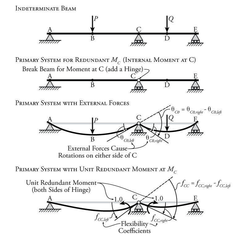
Similarly to the external reaction redundant case that was discussed previously, the internal redundant force method analysis shown in Figure 8.9 relies on the fact that we have some knowledge of the compatibility of the structure. In this case, the first step is to remove the continuity in the slope of the beam that is associated with the redundant internal moment at point C by adding a hinge at that point (which cannot transfer moment). Continuity in the slope at point C simply means that the slope is the same on the left side of C as it is on the right side of C. This slope continuity is the compatibility information that we will rely on for the force method analysis. We know that the full beam structure actually has a continuous slope at C, i.e. no 'kink'. So, to solve the problem we remove the internal moment restraint by adding a hinge, find out how much the beam will rotate on either side of the hinge due to the external forces, and then find out how much redundant force (in this case internal moments at point C) we need to add to the beam to counteract the external forces and make the slope at point C continuous again (to eliminate the kink).
Starting with the primary system with the added hinge (second from the top in Figure 8.9), we first add the external forces and see how much rotation we get on either side of the newly added hinge. We can find this rotation using any of the methods from Chapter 5. This rotation may be different on the left side of C ($\theta_{C0,left}$) and right side of C ($\theta_{C0,right}$) as shown. Note that, in this case as drawn in the figure, $\theta_{C0,left}$ is a positive rotation (counter-clockwise), and $\theta_{C0,right}$ is a negative rotation (clockwise). The total amount of kink at point C ($\theta_{C0}$ as shown in the figure) can be measured as the difference of these two rotations:
\begin{equation} \boxed{ \theta_{C0} = \theta_{C0,right} - \theta_{C0,left} } \label{eq:rel-rot} \tag{1} \end{equation}
This is equal to the total change in slope/rotation of the beam from the left side of C to the right side of C.
This total change in rotation must be counter-acted by the redundant force, which must bring the beam back to straight and eliminate the kink. We know that there must not be any kink or instantaneous change in slope because the real beam is continuous. So we apply a redundant internal moment at C as two opposite direction unit moments, one on either side of point C (as shown at the bottom of Figure 8.9). These moments are applied in the positive sense according to our sign convention from Chapter 1. Unit moments are used because we don't actually know the magnitude of the internal moment at C. Like the external reaction redundant case, we will find the rotation caused by the redundant in terms of a flexibility, so that we know how much rotation is caused by a single unit of moment. From that, we can use the compatibility relationship to solve for the unknown redundant moment, as we will see. These unit moments are unitless (i.e. they are not in units of $\mathrm{kNm}$). Two unit moments are required because if we cut a continuous beam at a single location, the internal moment would be represented by equal and opposite moments on either side of the cut (as previously discussed in Chapter 1). The resulting rotation on either side of the cut caused by the pair of redundant internal unit moment (which are our flexibilities) are $f_{CC,left}$ and $f_{CC,right}$ as shown in the figure. Similar to before, as shown, $f_{CC,left}$ is positive, and $f_{CC,right}$ is negative. In this notation '$CC$' the first letter is the location that the deflection or rotation (flexibility) is measured at and the second letter is the location of the unit load or moment that is causing that deflection or rotation. In this case, the flexibility and unit moment are located at the same position C, hence '$CC$'. Like the situation for the primary system with the external load, when we add the redundant unit moments here, we are interested in the total relative change in rotation from the left side of point C to the right side:
\begin{equation} \boxed{ f_{CC} = f_{CC,right} - f_{CC,left} } \label{eq:rel-flex} \tag{2} \end{equation}
This total change in slope of the beam from the left side of C to the right side of C is what will counteract the total difference in slope caused by the external forces when we apply our compatibility condition. Note that in this case, the redundant internal moments shown in Figure 8.9 do not appear to be counteracting the external loads, since they both cause rotations/deflections in the same direction. This is not a problem, it only means that our assumption for the direction of the internal redundant moment (positive) is not correct. This will come out of the compatibility equation when the internal moment redundant $M_C$ comes out as a negative number.
To find the amount of internal moment $M_C$ that will cause the primary beam to become continuous at point C again (to make sure that there is no kink), we must apply the following compatibility condition:
\begin{align} (\theta_{C0,right} - \theta_{C0,left}) + (f_{CC,right} - f_{CC,left}) M_C = 0 \tag{3} \end{align}
where $M_C$ is our redundant moment, the parameter that we are trying to find using the force method. Applying equations \eqref{eq:rel-rot} and \eqref{eq:rel-flex}, we get:
\begin{equation} \boxed{ \theta_{C0} + f_{CC} M_C = 0 } \tag{4} \end{equation}
The rotation $\theta_{C0}$ and the flexibility $f_{CC}$ are found through the analysis of the primary system, leaving $M_C$ as the only unknown:
\begin{equation} \boxed{M_C = -\frac{\theta_{C0}}{f_{CC}} } \tag{5} \end{equation}
Example
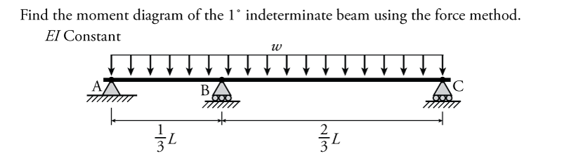
The use of the force method of analysis with an internal redundant force will be illustrated using the example in Figure 8.10. This is a ${1^\circ}$ indeterminate multi-span beam structure with a uniform distributed load $w$ along it's entire length. Find the moment diagram in terms of the distributed load value $w$ and the total beam length $L$. The $EI$ of the beam is constant along the length.
Similar to the structure in the previous discussion, the internal moment at the centre support $M_B$ will be used as the redundant force for the force method analysis of this beam. To form the primary system, the continuity associated with the internal moment $M_B$ must be removed by adding a hinge at point B. The resulting primary system is shown at the top of Figure 8.11.
The next step in this problem is to identify the appropriate compatibility condition/equation. The compatibility condition for this system will be that the beam must have a continuous slope at point B, which may be represented by the equation:
\begin{equation*} \theta_{B0} + f_{BB} M_B = 0 \end{equation*}
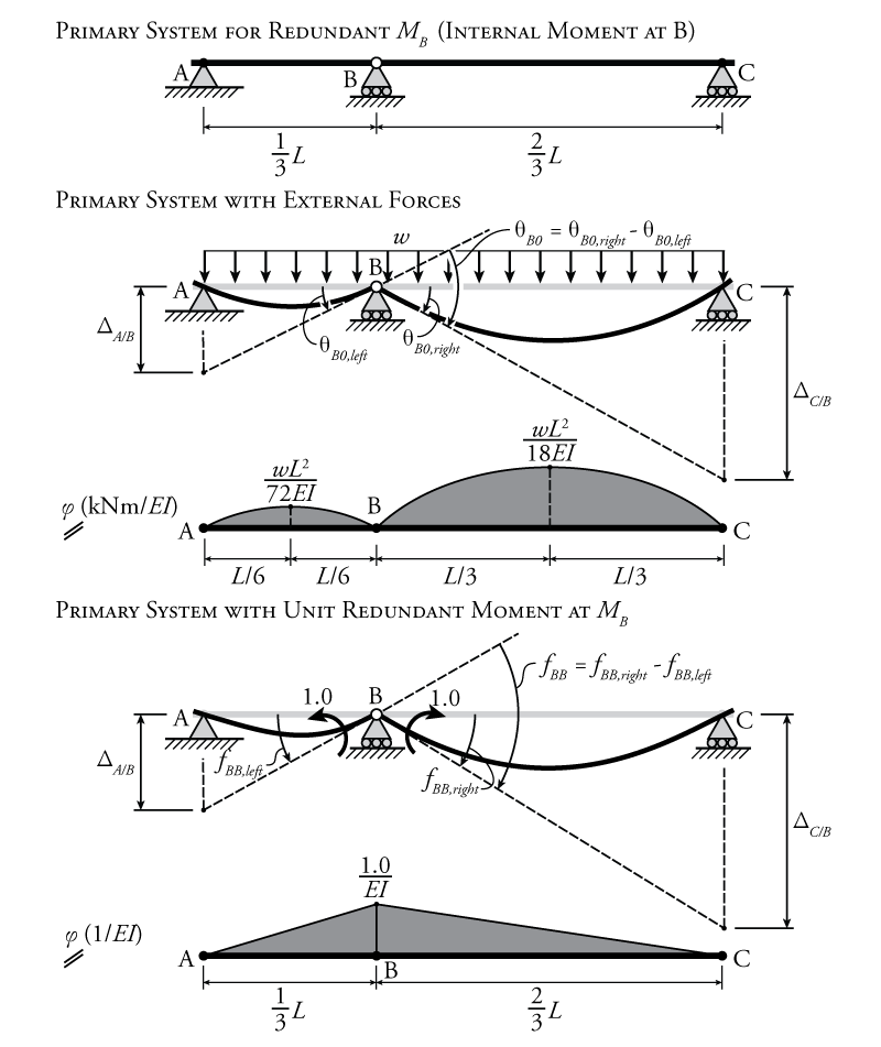
The first step in the analysis is to find the effect of the external beam loads (in this case the distributed load $w$) on the rotation of the beam on the left and right sides of the new hinge at point B. This situation is shown in Figure 8.11 (Primary System with External Forces). The distributed load causes the primary system to deflect downwards for each span as if each span was a separate simply-supported beam. This causes rotations $\theta_{B0,left}$ and $\theta_{B0,right}$ at point B as shown on the figure. The resulting curvature diagram for the primary system with the external load is also shown on the figure.
The rotations $\theta_{B0,left}$ and $\theta_{B0,right}$ may be determined using any of the methods from Chapter 5. In this example, we will use the second moment area theorem. The second moment area deviations ($\Delta_{A/B}$ and $\Delta_{C/B}$), from the tangent at B to the deflected shape at the supports on the left and right ends of the beam, are shown in Figure 8.11. Recall that these are found by calculating the moment of the area of the curvature diagram between the deflected point and the location associated with the reference tangent. Also recall from Figure 5.7 in Chapter 5 that the area of the half parabolas in our curvature diagram will be $\frac{2}{3}LM$ and the centroid of that area is $\frac{3}{8}L$ from the high side of the parabola. Knowing these, we can apply the second moment area theorem to find the rotations $\theta_{B0,left}$ and $\theta_{B0,right}$ (don't forget that the moment arms for the areas are always measured relative to the deflected point, not the reference tangent point):
\begin{align*} \Delta_{A/B} &= \left[ \frac{2}{3} \left(\frac{L}{6} \right) \left( \frac{wL^2}{72EI} \right) \right] \left[ \frac{5}{8} \left(\frac{L}{6} \right) \right] + \left[ \frac{2}{3} \left(\frac{L}{6} \right) \left( \frac{wL^2}{72EI} \right) \right] \left[ \frac{L}{6} + \frac{3}{8} \left(\frac{L}{6} \right) \right] \\ \Delta_{A/B} &= \frac{wL^4}{1944EI} \\ \therefore \theta_{B0,left} &= \frac{\Delta_{A/B}}{L/3} \end{align*} \begin{equation*} \boxed{ \theta_{B0,left} = \frac{wL^3}{648EI} } \end{equation*}
For $\theta_{B0,right}$:
\begin{align*} \Delta_{C/B} &= \left[ \frac{2}{3} \left(\frac{L}{3} \right) \left( \frac{wL^2}{18EI} \right) \right] \left[ \frac{5}{8} \left(\frac{L}{3} \right) \right] + \left[ \frac{2}{3} \left(\frac{L}{3} \right) \left( \frac{wL^2}{18EI} \right) \right] \left[ \frac{L}{3} + \frac{3}{8} \left(\frac{L}{3} \right) \right] \\ \Delta_{C/B} &= \frac{2wL^4}{243EI} \\ \therefore \theta_{B0,right} &= -\frac{\Delta_{C/B}}{2L/3} \end{align*} \begin{equation*} \boxed{ \theta_{B0,right} = -\frac{wL^3}{81EI} } \end{equation*}
The directions of the rotations $\theta_{B0,left}$ and $\theta_{B0,right}$ were determined through inspection of the deflected shape of the beams in Figure 8.11. For $\theta_{B0,right}$, the rotation is negative because it is clockwise. If virtual work was used to find these rotations instead, then the direction of the final rotation would be relative to the assumed direction of the unit point moment.
Using equation \eqref{eq:rel-rot}, we can find the total change in slope (amount of kink) between the left side and right side of point B:
\begin{align*} \theta_{B0} &= \theta_{B0,right} - \theta_{B0,left} \\ \theta_{B0} &= -\frac{wL^3}{81EI} - \frac{wL^3}{648EI} \end{align*} \begin{equation*} \boxed{ \theta_{B0} = -\frac{wL^3}{72EI} } \end{equation*}
This gives us one ingredient for our compatibility condition equation.
The next required ingredient for the compatibility condition is the flexibility of the primary system at point B due to the unit redundant moments as shown in the lower part of Figure 8.11. To find this flexibility, a pair of unit moments is added to either side of the newly added hinge at point B of the primary system as shown in the figure. The unit moment on the left side is counter-clockwise and the unit moment on the right side is clockwise. These are equal and opposite and both together represent a positive internal moment in the beam (which causes the beam to bend such that it is concave-up on either side of B).
The resulting curvature diagram for the primary system subject to the unit redundant moments is shown at the bottom of Figure 8.11. We can use this curvature diagram with the second moment area theorem to find the rotations on the left and right of point B caused by the unit redundant moments ($f_{BB,left}$ and $f_{BB,right}$), which are our flexibility coefficients:
\begin{align*} \Delta_{A/B} &= \left[ \frac{1}{2} \left( \frac{L}{3} \right) \left( \frac{1.0}{EI} \right) \right] \left[ \frac{2}{3} \left( \frac{L}{3} \right) \right] \\ \Delta_{A/B} &= \frac{L^2}{27EI} \\ \therefore f_{BB,left} &= \frac{\Delta_{A/B}}{L/3} \end{align*} \begin{equation*} \boxed{ f_{BB,left} = \frac{L}{9EI} } \end{equation*}
Again, the calculation for $f_{BB,right}$ is similar but has a negative rotation:
\begin{align*} \Delta_{C/B} &= \left[ \frac{1}{2} \left( \frac{2L}{3} \right) \left( \frac{1.0}{EI} \right) \right] \left[ \frac{2}{3} \left( \frac{2L}{3} \right) \right] \\ \Delta_{C/B} &= \frac{4L^2}{27EI} \\ \therefore f_{BB,right} &= -\frac{\Delta_{C/B}}{2L/3} \end{align*} \begin{equation*} \boxed{ f_{BB,right} = -\frac{2L}{9EI} } \end{equation*}
and using equation \eqref{eq:rel-flex}, we can find the total change in slope (amount of kink) between the left side and right side of point B:
\begin{align*} f_{BB} &= f_{BB,right} - f_{BB,left} \\ f_{BB} &= -\frac{2L}{9EI} - \frac{L}{9EI} \end{align*} \begin{equation*} \boxed {f_{BB} = -\frac{L}{3EI} } \end{equation*}
This gives us the last ingredient for our compatibility condition equation.
Applying our compatibility equation now, we can solve for the unknown internal moment redundant $M_B$:
\begin{align*} \theta_{B0} + f_{BB} M_B &= 0 \\ M_B &= -\frac{\theta_{B0}}{f_{BB}} \\ M_B &= - \left(-\frac{wL^3}{72EI} \right) \left(-\frac{3EI}{L} \right) \end{align*} \begin{equation*} \boxed {M_B = -\frac{wL^2}{24} } \end{equation*}
Now that we know the moment at point B ($M_B$), we can go back to the full structure and solve for the reactions, as shown in Figure 8.12. The full free body diagram of the structure is shown near the top of the figure. We can see immediately that the horizontal reaction at point A ($A_x$) will be zero due to horizontal equilibrium. The force method analysis did not give us any information about the full global free body diagram; however, if we make a cut in the free body diagram at point B, we know the internal moment at the cut section $M_B$, which was our redundant force in the analysis.
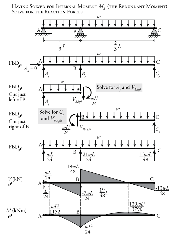
If we take a free body diagram of a cut at point B just to the left of point B as shown in Figure 8.12, we can use a moment equilibrium around point B to find the reaction $A_y = \frac{1}{24}wL \uparrow$. Since the solved internal moment $M_B$ is negative, the moment arrow on the right side of member AB for this cut section will be clockwise (to cause concave-down style bending). We take the cut just to the left of point B so that our free body diagram does not include the vertical reaction at B ($B_y$). This allows us to use vertical equilibrium to also find the shear just to the left of point B which is $V_{B,left} = -\frac{7}{24}wL$. The shear to the left of B is negative because the arrow for $V_B$ will point up. Recall that our sign convention is that shear arrows that point up on the right side of a member represent negative shear. Recall as well that the shear force is undefined right at the position of an external reaction force because the reaction changes the shear instantaneously at that point. Therefore, it is only useful to talk about the shear 'just to the left' or 'just to the right' of a reaction.
The same process may be followed for the right side of the beam (with a cut section just to the right of point B as shown in Figure 8.12) to give us the vertical reaction $C_y = \frac{13}{48}wL \uparrow$ and shear to the right of B which is $V_{B,right} = \frac{19}{48}wL$. The last missing piece, the vertical reaction $B_y$ can be found using global equilibrium to be $B_y = \frac{21}{24}wL \uparrow$. The completed free body diagram with the known reactions is shown in the figure, and this may be used to draw the final shear and moment diagrams for the indeterminate multi-span beam as shown.
Trusses
The use of an internal redundant force is also common for indeterminate truss analysis. Any truss system with dual cross-braces, such as the one shown at the top of Figure 8.13 will be internally indeterminate. This particular truss also happens to be externally determinate since it only has three external reaction components. This means that the only way to find the forces in this truss using the force method is to use an internal truss axial force as a redundant. If we removed a reaction component to use as the redundant, then the resulting primary system would be unstable (and therefore, impossible to analyse).
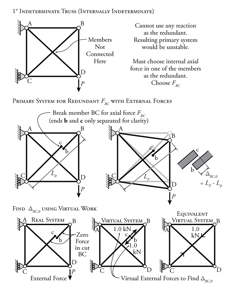
When using a truss member internal axial force as the redundant force for a force method analysis, we need to release the deformation associated with the axial force. This means that we must effectively completely break the truss member to form the determinate primary system, since truss members only resist axial forces. It does not matter where along the truss member we break it. We will consider that the remaining pieces of the truss member remain in place, even though they would technically fall out of place when the member cut in the middle.
For the single degree of indeterminacy truss shown in Figure 8.13, the force method analysis process will be illustrated using the axial force in truss member BC ($F_{BC}$) as the redundant. The resulting primary system for this truss is shown in the middle of Figure 8.13. Member BC is cut at a single point along its length and the cut ends are labelled b and c. When the external force is applied, as shown in the figure, the truss deforms and the BC diagonal distance, originally $L_0$ is shortened to $L_P$. This causes the newly cut ends at b and c to overlap as shown in the image on the right side of the figure. We can call the length of the overlap due to the external force $\Delta_{BC,0}$ which is equal to the difference between the initial length of the diagonal BC ($L_0$) and the final length after the application of external force $P$ ($L_P$).
To find the value of the overlap $\Delta_{BC,0}$ we can use the method of virtual work from Chapter 5. The real system for this virtual work analysis is simply the primary system with the external load applied (and no force in members Cc and Bb since they are no longer connected axially). This is a determinate truss that is easy to analyse. The virtual system will be the same primary system, without the external force $P$, but instead with virtual external unit loads applied at each cut end at b and c. This pair of virtual unit loads is in the same location and direction as the unknown that we want to find, i.e. the overlap of the two cut ends at b and c. Having two unit loads in opposite directions instead of a single unit load will mean that the virtual work method will result in the relative movement of the two ends instead of the absolute deflection of either end. The real and virtual systems for finding $\Delta_{BC,0}$ are shown at the bottom of Figure 8.13.
The virtual system, with unit loads at points b and c, shown at the bottom middle of Figure 8.13, is also equivalent to the virtual system shown at the bottom right of the figure. The unit loads at b and c put both cut members Bb and Cc into an equal $1.0\mathrm{\,kN}$ of tension. So we can easily conceptualize and analyse the truss virtual system as if the member BC was not cut but had a known axial tension of $1.0\mathrm{\,kN}$ as shown at the bottom right of the figure.
As we have just seen, in the primary system subject to the external load, the load causes the two cut ends of the member BC to overlap by $\Delta_{BC,0}$, an amount which we can calculate using virtual work. In the full indeterminate system, we know that the member BC cannot overlap itself because it is actually continuous and not cut. Therefore, we need to find the value of the redundant internal axial force in member BC ($F_BC$) that will counteract this overlap by pushing the split ends of the member at b and c apart. Again, as in previous analyses, we will find the effect on the overlap caused by a unit redundant load to find a flexibility coefficient. This flexibility coefficient will be a measure of how much the two cut ends b and c would overlap each other for each unit of axial force applied at the cut ends. This will allow us to determine how much force in member BC in the primary system will exactly counteract the overlap caused by the external forces.
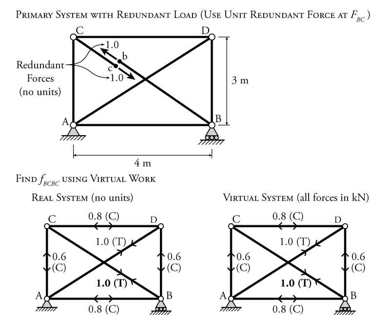
To find the flexibility coefficient, we will apply unit redundant loads to members Bb and Cc at both cut points (at points b and c) as shown in Figure 8.14. Like the internal moment redundant for the beam that was discussed in the previous section, we need a pair of forces to represent the action of the internal axial force. This is because the internal axial force causes forces that are equal and opposite at any cut section. These unit redundant forces will cause the truss to deform and will create their own overlap at the cut section as shown at the top right of Figure 8.14. This overlap caused by the unit redundant forces is our flexibility coefficient $f_{BCBC}$. In this notation, '$BCBC$' the first pair of letters is the location that the overlap is measured at and the second pair of letters is the location of the unit internal axial load. In this case, the overlap (flexibility) and unit internal axial load are for the same member BC, hence '$BCBC$'.
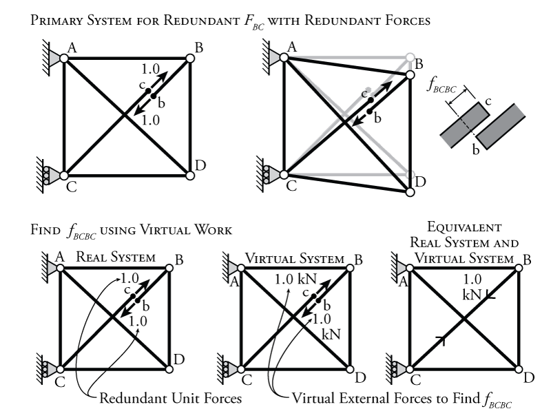
Since we will consider the unit redundant to represent a tension force (because we generally tension axial forces to be positive), the resulting flexibility coefficient $f_{BCBC}$ will represent an overlap of the cut ends as shown on the right side of Figure 8.14; this means that when we apply our compatibility condition, the force in BC will need to come out negative in order to counteract the effect of the external forces. The redundant force in this case will have to produce a gap between the ends b and c to compensate for the overlap caused by the external forces on the primary system.
To find the value of the flexibility coefficient (the amount of overlap caused by a unit amount of redundant force), we can again use virtual work as shown on the bottom of Figure 8.14. The real system for the virtual work is our primary system with the unit redundants on either side of the cut at point b and c as shown in the figure (but with no units for the redundants). The virtual system is identical since we are trying to find the overlap at that location (the same thing we were trying to do previously for the primary system with the external load). Both the real and virtual systems cause a uniform unit tension force in both cut pieces Bb and Cc and so, as before, can both be analysed as if the member BC was not cut but instead had a known axial tension of $1.0\mathrm{\,kN}$ (or just $1.0$ for the real system) as shown at the bottom right of Figure 8.14. The real and virtual system here are the same as the virtual system for the primary system with the external load (the one shown at the bottom right of Figure 8.13. This means that we can use the same truss solution for all three. This virtual work analysis gives us the flexibility coefficient $f_{BCBC}$.
Now, since we know that the total redundant force $F_{BC}$ needs to compensate for the overlap caused by the external force on the primary system ($\Delta_{BC,0}$), we can use compatibility to solve for that redundant as before:
\begin{equation} \boxed{ \Delta_{BC,0} + f_{BCBC} F_{BC} = 0 } \tag{6} \end{equation}
where $\Delta_{BC,0}$ is the overlap or gap between cut ends b and c in the primary system caused by the external force on the truss, $f_{BCBC}$ is the overlap or gap between cut ends b and c in the primary system caused by the unit redundant internal axial force at the location of the cut ends, and $F_{BC}$ is the total redundant internal axial force in member BC. If $\Delta_{BC,0}$ causes an overlap between b and c, then $F_{BC}$ must create an equal and opposite gap between b and c that is equal to:
\begin{equation} \Delta_{BCBC} = f_{BCBC} F_{BC} = -\Delta_{BC,0} \tag{7} \end{equation}
Example
The force method process for trusses with a single degree of internal indeterminacy will be illustrated using the example structure shown in Figure 8.15. This is an indeterminate truss with a single external point load of $100\mathrm{\,kN}$.
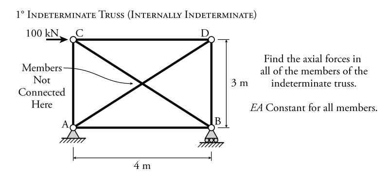
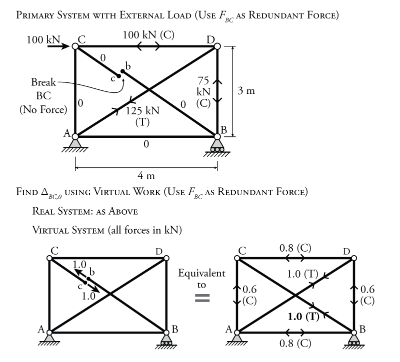
The first step in the analysis is to select a redundant. For this example, we will select the internal axial load in member BC as the redundant force. This is an internal redundant. This will require the continuity associated with the internal axial redundant force to be removed, resulting in the primary system shown at the top of Figure 8.16. To remove the continuity effect of the redundant, we have to make member BC unable to resist an internal axial force, which means that we must break the axial resistance of the member anywhere between its ends. In this example, the member BC is broken at points b and c as shown in the figure. For the solution, it does not matter where along the member points b and c are located. We will consider that, although the member is broken for axial at points b and c, the broken ends of the member will stay in place so that we can see how much they overlap or separate when load is applied to the primary system.
We will use the primary system to find the required ingredients for our compatibility condition, with the ultimate goal of solving for our redundant force so that we reduce the indeterminate truss system to a determinate system that we can solve using the method of joints. With the internal axial force in member BC as our redundant, the compatibility condition for this example structure is:
\begin{equation*} \Delta_{BC,0} + f_{BCBC} F_{BC} = 0 \end{equation*}
where $\Delta_{BC,0}$ is the overlap or gap between the cut section ends b and c caused by the external forces, $f_{BCBC}$ is the overlap or gap between the cut section ends b and c caused by the unit redundant force, and $F_{BC}$ is the magnitude of the redundant force (which we are trying to solve for).
The first load that we will apply to the primary system is the external load, in this case the $100\mathrm{\,kN}$ load at point C, as shown in Figure 8.16. We would like to measure how much the cut ends of member BC will overlap when that load is applied ($\Delta_{BC,0}$). To do this, we will use virtual work on the primary system with the external load. The real system is simply the primary system with the external load. Since member BC is cut and there is no external load directly applied to that member, the load in BC will be zero and we can ignore it. The rest of the truss member forces may be found using the method of joints, with the resulting forces shown in the upper diagram in Figure 8.16.
As discussed previously, the virtual system to find the overlap of b and c is the primary system with a pair of unit loads applied to the cut ends as shown in the lower half of Figure 8.16. This system may be solved by considering the load in member BC to be $1.0\mathrm{\,kN}$ in tension before starting the analysis. This $1.0\mathrm{\,kN}$ load is shown in bold in the figure. Even though the system shown is indeterminate because of the cross-brace. Once we know the force in one of the members is $1.0\mathrm{\,kN}$, we have enough information to solve the forces in all of the other members using the method of joints. The resulting forces in all of the members of the virtual system are shown in the figure.
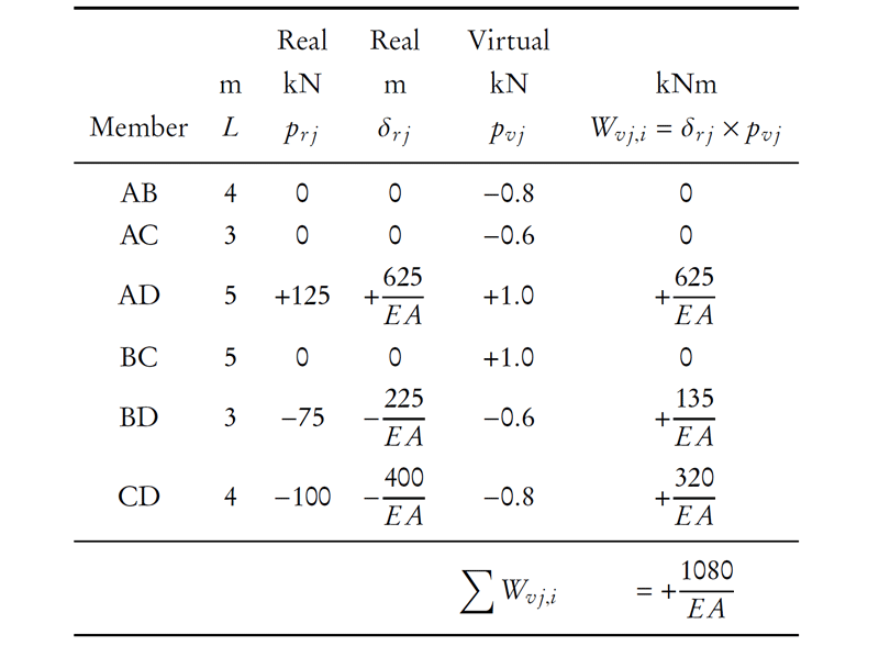
Knowing the real and virtual system forces in all of the members, we can apply virtual work to find the overlap of b and c ($\Delta_{BC,0}$) as shown in Table 8.1.
Applying the virtual work balance:
\begin{align*} W_{v,e} &= W_{v,i} \\ (1\mathrm{\,kN})(\Delta_{BC,0}) &= \frac{{1080}}{EA} \; \mathrm{kNm} \\ \Delta_{BC,0} &= \frac{{1080}}{EA} \; \mathrm{m} \end{align*}
which is the overlap of points b and c caused by the external load on the primary system.
The next step is to find the effect of the unit redundant internal axial force. This unit redundant force is applied at the cut ends b and c as shown in Figure 8.17. This force is unitless. To find the flexibility coefficient $f_{BCBC}$ we can use virtual work to find the overlap of points b and c caused by the unit redundant forces. The real and virtual systems for this virtual work analysis are the same as the virtual system for the primary system subjected to the external force previously shown in Figure 8.16.
Knowing the real and virtual system forces in all of the members, we can apply virtual work to find the overlap of b and c ($f_{BCBC}$) as shown in Table 8.2.
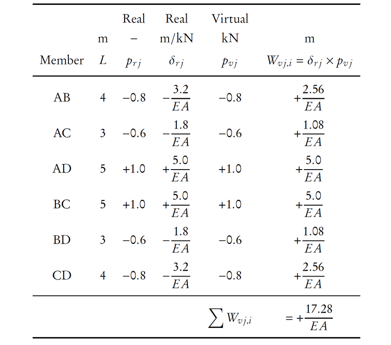
Applying the virtual work balance:
\begin{align*} W_{v,e} &= W_{v,i} \\ (1\mathrm{\,kN})(f_{BCBC}) &= \frac{{17.28}}{EA} \; \mathrm{m} \\ f_{BCBC} &= \frac{{17.28}}{EA} \; \mathrm{m/kN} \end{align*}
which is the overlap of points b and c caused by the redundant load on the primary system (per $\mathrm{kN}$ of redundant load).
Now that we have solved for $\Delta_{BC,0}$ and $f_{BCBC}$, we can use the compatibility equation for the system to solve for the redundant force magnitude $F_{BC}$:
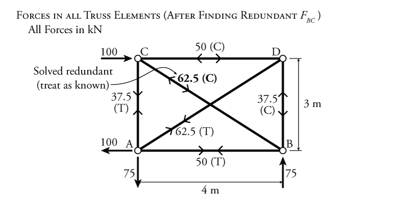
\begin{align*} \Delta_{BC,0} + f_{BCBC} F_{BC} &= 0 \\ F_{BC} &= -\frac{\Delta_{BC,0}}{f_{BCBC}} \\ F_{BC} &= - \left( \frac{{1080}}{EA} \; \mathrm{m} \right) \left( \frac{EA}{{17.28}} \; \mathrm{kN/m} \right)\\ F_{BC} &= -62.5\mathrm{\,kN} \\ F_{BC} &= 62.5\mathrm{\,kN} \; \text{(Compression)} \end{align*}
Going back to the full system now, with the redundant force in member BC included in the truss as a known force, the rest of the truss member axial forces may be found. This complete truss solution is shown in Figure 8.18.