 Learn About Structures
In the previous sections, we have looked at how to solve indeterminate systems with only one degree of indeterminacy (either internal or external determinacy). But, what happens if we have a system that has two or more degrees of indeterminacy? Such a situation is depicted in Figure 8.19. This beam is similar to the indeterminate beam studied previously in Figure 8.1, but with a fixed end at point A instead of a pin. This gives the beam an extra degree of indeterminacy, making it a ${2^\circ}$ indeterminate system.
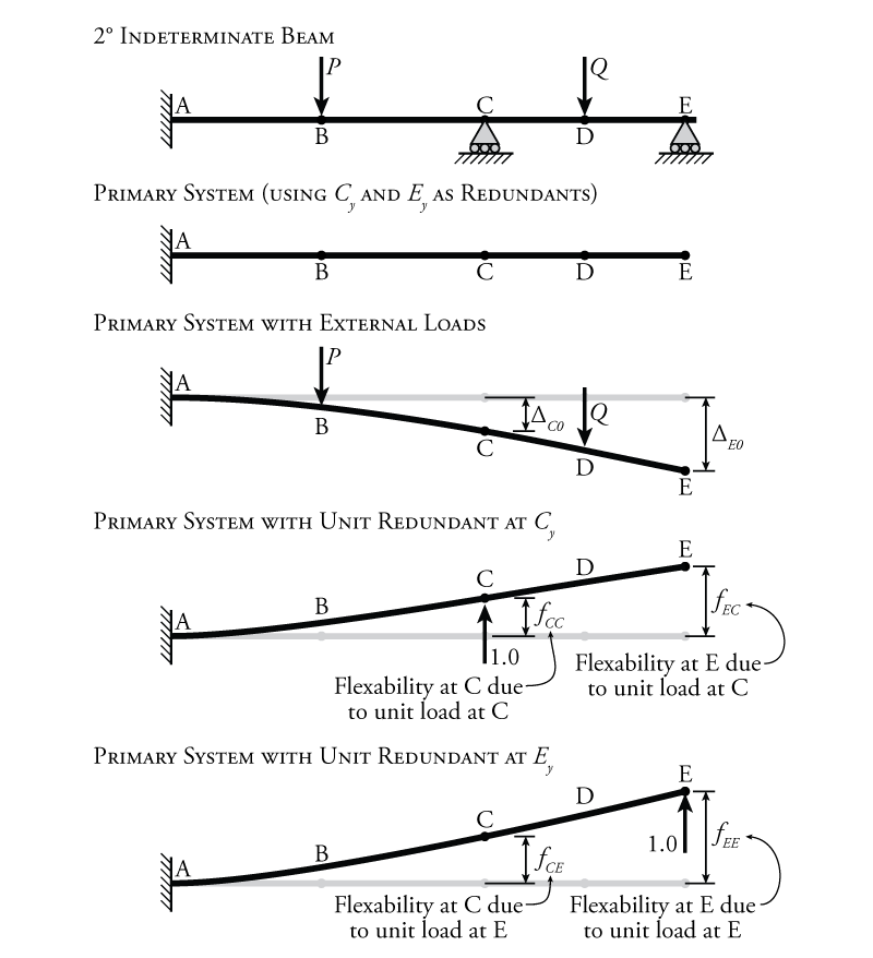
For every degree of indeterminacy, we must have a redundant force (internal or external). This is because, for a force method analysis, our primary system must be determinate (i.e the beam with the redundant restraints removed). For the example beam shown in Figure 8.19, we must select two different redundant forces because the beam is ${2^\circ}$ indeterminate. If we select the vertical reactions at points C and E ($C_y$ and $E_y$) as the redundants, as shown in the figure, then our primary system, with the redundant reactions removed, is determinate (it has become a simple cantilever).
Now that we have multiple redundant forces, we will have multiple compatibility conditions as well, one for each redundant. In the example beam in Figure 8.19, there is a compatibility condition associated with each support, i.e. that the overall displacement at the support has to equal zero.
To apply these two compatibility conditions, like before, we must separately consider the effect of the external loads and the redundant loads on the primary system. We will need to find the effect of each load (external and each redundant) on the deflections/rotations at the compatibility condition locations. This is shown for the external loads on the example structure in the middle of Figure 8.19. Since we have a compatibility equation for each reaction (that the support must remain at zero displacement), we need to know how the external forces on the primary system will effect the deflection of the beam at both of those support locations. These are shown in the figure as $\Delta_{CO}$ for the reaction location at point C and $\Delta_{E0}$ for the reaction location at point E. These deflections may be found by using any of the applicable methods from Chapter 5. Since this example is a determinate cantilever, it may be convenient to find the deflections using the moment area theorems for this problem.
With our previous force method analyses, we would then find the effect of a unit redundant (at the location of the redundant force) on the deflection at the same support location. We then used that unit redundant to find the total redundant force that is necessary to counteract the effect of the external loads on the primary system (to bring the support deflection back to zero, where we know it has to be because of compatibility).
When we have multiple redundants, we need to find the effect of each redundant force separately by analysing the structure separately for each one (one unit redundant force at each redundant force location). This results in two different redundant force analyses in addition to the analysis of the beam with the external load, as shown for our example in the lower two diagrams in Figure 8.19. Of course, each unit redundant load does not only effect the deflection of the structure at its own location, but also effects the deflection of the structure at the other unit redundant location. This is shown in the figure. For example, when a unit redundant load is applied at point C in the figure, this loads causes the entire beam to deflect. In particular, we are interested in how much the beam deflects at the two redundant load (support) locations. When the unit redundant is applied at point C (the second diagram from the bottom in Figure 8.19), the deflection of the beam at point C is called $f_{CC}$, which is the flexibility at point C when the unit load is applied at point C. Likewise, that same unit load at point C also causes deflection of the beam at point E called $f_{EC}$ which is the flexibility at point E when the unit load is applied at point C. When the unit load is applied at point E (the bottom diagram in Figure 8.19), the deflection of the beam at point E is called $f_{EE}$, which is the flexibility at point E when the unit load is applied at point E. Likewise, that same unit load at point E also causes deflection of the beam at point C called $f_{CE}$ which is the flexibility at point C when the unit load is applied at point E.
We can find all of these flexibility terms explicitly using the methods from Chapter 5. The difference for multiple redundants is that we now must solve one system for each redundant, and for each of those systems, we must find as many deflections as there are redundants. This means the total number of deflections we have to solve is equal to the square of the number of redundants! Clearly this shows that the amount of work for a force method analysis will increase exponentially as the number of redundants (and therefore, degrees of indeterminacy) increases. We can save a bit of this work by taking advantage of Maxwell's Law of Reciprocal Deformations as we shall see later; however, it is clear that the force method will become quite unmanageable for indeterminate systems with many degrees of indeterminacy.
Once we have all of our flexibility terms (for our example, $f_{CC}$, $f_{EC}$, $f_{EE}$, and $f_{CE}$), and all of our primary system deflections due to the external loads (in our example, $\Delta_{CO}$ and $\Delta_{E0}$), then we can apply our compatibility conditions to solve for the redundant forces. For the example structure in Figure 8.19, there are two different compatibility conditions, one for each redundant reaction point where we know that the deflection must equal zero:
\begin{align} \Delta_{CO} + f_{CC} C_y + f_{CE} E_y &= 0 \tag{1} \\ \Delta_{EO} + f_{EC} C_y + f_{EE} E_y &= 0 \tag{2} \end{align}
As can be seen in Figure 8.19, there are three different deflections that effect the displacement at point C in the primary system: the deflection at C caused by the external loads ($\Delta_{CO}$), the deflection at C caused by the redundant load at point C ($\Delta_{CC}= f_{CC} C_y$), and the deflection at C caused by the redundant load at point E ($\Delta_{CE}= f_{CE} E_y$). Note that the last one is dependent on the amount of redundant load that is applied at point E, not the redundant applied at point C. Likewise, there are three other deflections that effect the displacement at point E in the primary system: the deflection at E caused by the external loads ($\Delta_{EO}$), the deflection at E caused by the redundant load at point C ($\Delta_{EC}= f_{EC} C_y$), and the deflection at E caused by the redundant load at point E ($\Delta_{EE}= f_{EE} E_y$).
Once we have the above equations set up, we can use simple determinate analyses of the three different primary systems in Figure 8.19 to find numerical deflection values for all of the parameters except for the redundant force magnitudes $C_y$ and $E_y$. Since we have two equations and two unknowns, these unknown magnitudes $C_y$ and $E_y$ may be found easily by rearranging one equation in terms of one of the parameters and then subbing that result into the other equation to solve. As the number of degrees of indeterminacy of a problem increases, the number of redundant forces and the number of compatibility conditions increase accordingly. So, for a ${3^\circ}$ indeterminate structure, using the force method, we would have to solve a system of three equations and three unknowns.
Like before, once we have found the values for all of the redundants, we can go back to our full system, treat those redundant forces as known forces, and solve the rest of the system using equilibrium only.
Maxwell's Law of Reciprocal Deformations
In the previous example, we had to find four different flexibility coefficients by analysing the determinate primary structure: $f_{CC}$, $f_{EC}$, $f_{EE}$, and $f_{CE}$. Using Maxwell's Law of Reciprocal Deformations we can cut that number down to three for this case. Maxwell's Law of Reciprocal Deformations states that, for a linear elastic structure, the deflection at a point B caused by a unit load at point A, is equal to the deflection at point A caused by a unit load at point B. For the previous example, this means that we could say that:
\begin{equation} f_{EC} = f_{CE} \tag{3} \end{equation}
So, we would only have to solve for one or the other, not both.
If we have a ${3^\circ}$ indeterminate structure with redundant loads at points A, B and C, then we need to find the effect of each redundant unit load on the deflections at all three locations. That is, we would need to find $f_{AA}$, $f_{AB}$, $f_{AC}$, $f_{BA}$, $f_{BB}$, $f_{BC}$, $f_{CA}$, $f_{CB}$, $f_{CC}$, nine different flexibility coefficients. Using Maxwell's Law of Reciprocal Deformations, we can say that:
\begin{align*} f_{AB} &= f_{BA} \\ f_{AC} &= f_{CA} \\ f_{BC} &= f_{CB} \end{align*}
This cuts our work down from finding nine flexibility coefficients, to just having to find six.
We can show that Maxwell's Law of Reciprocal Deformations works by applying virtual work. Recall from Chapter 5 that internal virtual work for a bending structure is equal to:
\begin{equation} W_{v,i} = \int_0^L \frac{M_v M_r}{EI} dx \tag{4} \end{equation}
where $M_v$ is the moment in the virtual system, $M_r$ is the moment in the real system, $E$ is the Young's Modulus of the member, and $I$ is the moment of inertia (second moment of area) of the member. Often, we consider that $\frac{M_r}{EI}$ is the curvature of the real system, but the $EI$ could just as easily be attached to the virtual system instead, it doesn't matter in this formulation. Likewise, the external virtual work is equal to the external displacements in the real system multiplied by the external forces in the virtual system:
\begin{equation} W_{v,e} = \sum_i \Delta_{ri} P_{vi} \tag{5} \end{equation}
where $\Delta_{ri}$ is the deflection of the real system at each location of a virtual external force $i$, and $P_{vi}$ is the external virtual force $i$. In typical virtual work analysis, we usually only have one virtual force, but this is equation is also valid for if we have multiple virtual forces, each being paired with its own real deflection at the location of that force.
Now, let's say that we have a real system (called system A) with $i$ different external forces, and a virtual system (called system B) with $j$ different external forces. Using the virtual work balance:
\begin{align} W_{v,e} &= W_{v,i} \tag{6} \\ \sum_j \Delta_{Aj} P_{Bj} &= \int_0^L \frac{M_B M_A}{EI} dx \tag{7}\end{align}
Each virtual external force $P_{Bj}$ is accounted for explicitly on the left side of the equation, as well as causing the moment $M_B$. Each real external force contributes to the deflection $\Delta_{Aj}$ at each virtual external force location, and together they cause the moment $M_r$.
Now let's switch the real and virtual system, system A will be the virtual system and system B will be the real system. We get the virtual work force balance:
\begin{align} W_{v,e} &= W_{v,i} \tag{8} \\ \sum_i \Delta_{Bi} P_{Ai} &= \int_0^L \frac{M_A M_B}{EI} dx \tag{9}\end{align}
Now notice that, while the left side of the equation has changed significantly, the right side is the same as it was before. Switching the position of $M_A$ and $M_B$ has no effect on the multiplication.
Since the right sides of the equations (the internal virtual work) are the same no matter which system we consider to be real and which we consider to be virtual, then:
\begin{align} \sum_j \Delta_{Aj} P_{Bj} = \sum_i \Delta_{Bi} P_{Ai} \tag{10} \end{align}
If we now consider the external forces from both system A and system B are virtual forces (unit loads $P_{Bj} = 1$, and $P_{Ai} = 1$), then:
\begin{align} \sum_j \Delta_{Aj}= \sum_i \Delta_{Bi} \tag{11} \end{align}
If we simplify this further, such that there is only one external load in system A and one external load in system B, then:
\begin{align} \Delta_{Aj} = \Delta_{Bi} \tag{12} \end{align}
Recall that $\Delta_{Aj}$ is now the deflection at point A due to the unit force at point B and $\Delta_{Bi}$ is now the deflection at point B due to the unit force at point A. So, restated:
\begin{align} f_{AB} = f_{BA} \tag{13} \end{align}
Example
The force method for a structure with multiple degrees of indeterminacy will be illustrated using the example structure shown in Figure 8.20. This is a ${3^\circ}$ indeterminate frame with a constant $E$, but varying $I$.
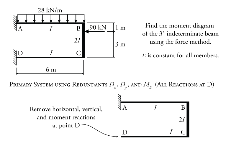
Since this frame is ${3^\circ}$ indeterminate, we must choose three redundant forces. To make the analysis of the primary structure easy, it is a good idea to select all three reactions at point D as the redundant forces ($D_x$, $D_y$ and $M_D$), as shown in Figure 8.20. This results in a primary system that is effectively a bent cantilever, which is easy to analyse.
So, the three compatibility conditions for this problem will be associated with the three support components at point D, and each compatibility condition will have four different contributors to the deflection/rotation at point D, one caused by the external loads on the primary system, and three more, one for each of the redundant unit forces in each reaction component direction at point D. The resulting compatibility conditions are:
\begin{align*} \Delta_{Dx,0} + f_{Dx,Dx}D_x + f_{Dx,Dy}D_y + f_{Dx,MD}M_D = 0 \\ \Delta_{Dy,0} + f_{Dy,Dx}D_x + f_{Dy,Dy}D_y + f_{Dy,MD}M_D = 0 \\ \Delta_{MD,0} + f_{MD,Dx}D_x + f_{MD,Dy}D_y + f_{MD,MD}M_D = 0 \end{align*}
where $\Delta_{Dx,0}$, $\Delta_{Dy,0}$ and $\Delta_{MD,0}$ are the deflections/rotations of the primary system at point D caused by the external loads on the structure, $D_x$ is the unknown horizontal redundant reaction at point D, $D_y$ is the unknown vertical redundant reaction at point D, $M_D$ is the unknown moment redundant reaction at point D, $f_{Dx,Dx}$ is the horizontal deflection at point D caused by a unit redundant force in the horizontal direction at point D, $f_{Dx,Dy}$ is the horizontal deflection at point D caused by a unit redundant force in the vertical direction at point D, $f_{Dx,MD}$ is the horizontal deflection at point D caused by a unit redundant moment at point D, etc.
We will have to find all of the parameters in the above equations except for the unknown redundant reaction forces/moments ($D_x$, $D_y$ and $M_D$) that we are trying to solve for. Of course, using Maxwell's Law of Reciprocal Deformations, we only need to find six out of the nine total flexibility coefficients. To find the values of the parameters, we can use virtual work. For the external load on the primary system, the virtual work analysis is illustrated in Figure 8.21. The primary system with the external loads (and the redundant reactions removed) is shown at the upper left of the figure. We can find the shear and moment diagrams as shown at the top right. Below that, the virtual systems for finding horizontal deflection at point D, vertical deflection at point D and rotation at point D are shown, along with their associated shear and moment diagrams. These three virtual systems are labelled System A, System B and System C, respectively as shown in the figure. Only the moment diagrams are shown here, not the curvature diagrams. The incorporation of the different element stiffness $EI$ to convert the moments to curvatures will be done later within the calculation of the internal virtual work.
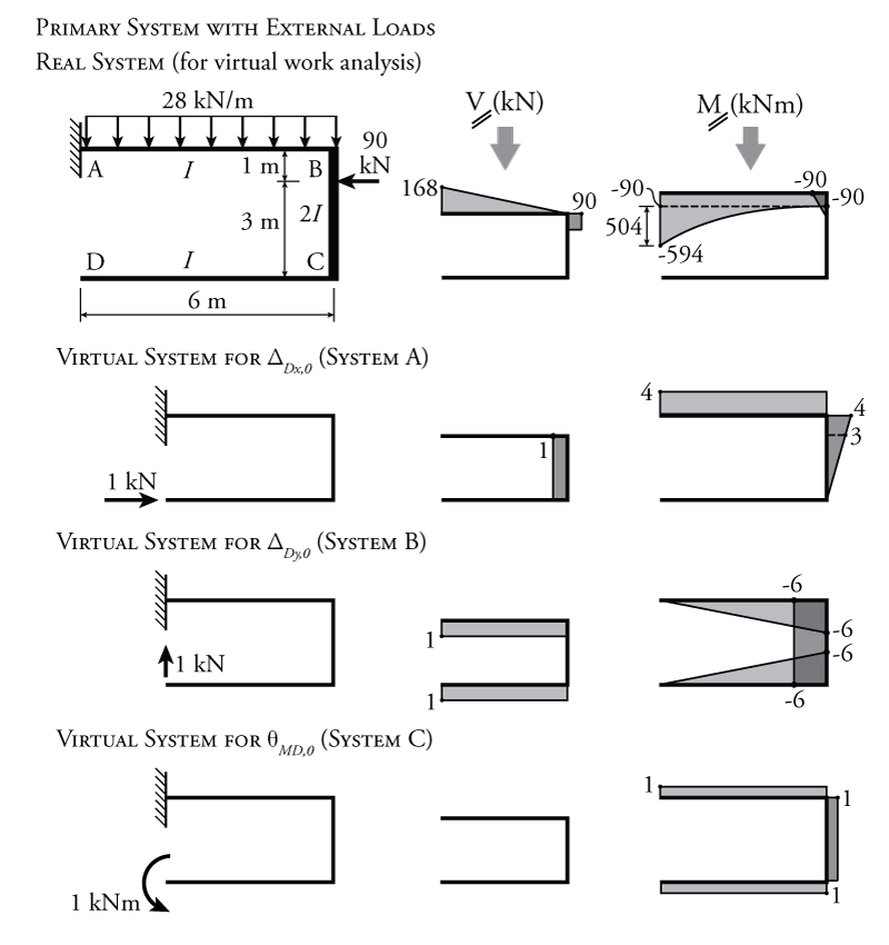
We can use a virtual work analysis to find the deflections at the redundant force locations caused by the external loads (using the virtual work product integration table from Figure 5.22) as shown below.
To find $\Delta_{Dx,0}$ using the External Load Moment Diagram (real system) with System A (virtual system) from Figure 8.21:
\begin{align*} W_{v,e} &= W_{v,i} \\ (1\mathrm{\,kN})(\Delta_{Dx,0}) &= (\textrm{rectangle 90})(\textrm{rectangle 4}) + (\textrm{parabola 504})(\textrm{rectangle 4}) \\ &\quad\quad + (\textrm{triangle 90})(\textrm{trapezoid 4,3}) \\ (1\mathrm{\,kN})(\Delta_{Dx,0}) &= \frac{1}{EI} \left[ LMQ \right] + \frac{1}{EI} \left[ \frac{LMQ}{3} \right] + \frac{1}{E2I} \left[ \frac{LM}{6} \left( 2Q_a + Q_b \right) \right] \\ (1\mathrm{\,kN})(\Delta_{Dx,0}) &= \frac{1}{EI} \left[ 6 (-90) (4) \right] + \frac{1}{EI} \left[ \frac{6(-504)(4)}{3} \right]\\ &\quad\quad + \frac{1}{E2I} \left[ \frac{1(-90)}{6} \left( 2(4) + (3) \right) \right] \\ \Delta_{Dx,0} &= \frac{-6274.5}{EI} \; \mathrm{m} \end{align*}
We had to divide the first leg of the real system (the one with the parabola) into two separate components to solve of the product integral using Figure 5.22. This is because the product integration table only has a parabola that goes from a maximum value to zero at a point of zero slope. So we must divide the leg up into a rectangle of height 90 and a parabola of height 504 as shown in Figure 8.21. Each of these components is integrated using the full height of the rectangle on the same leg of the virtual system A (of height 4). Since the virtual work product integral is a product of the moment in the real system (divided by $EI$ to get curvature) and the moment in the virtual system, this is equivalent to using the distributive property $A(B+C)=AB+AC$ inside the integral. Notice also that the higher moment of inertia $2I$ is taken into account within the third term of the long expression above.
To find $\Delta_{Dy,0}$ using the External Load Moment Diagram (real system) with System B (virtual system) from Figure 8.21:
\begin{align*} W_{v,e} &= W_{v,i} \\ (1\mathrm{\,kN})(\Delta_{Dy,0}) &= (\textrm{rectangle 90})(\textrm{triangle 6}) + (\textrm{parabola 504})(\textrm{triangle 6}) \\ &\quad\quad + (\textrm{triangle 90})(\textrm{rectangle 6}) \\ (1\mathrm{\,kN})(\Delta_{Dy,0}) &= \frac{1}{EI} \left[ \frac{LMQ}{2} \right] + \frac{1}{EI} \left[ \frac{LMQ}{12} \right] + \frac{1}{E2I} \left[ \frac{LMQ}{2} \right] \\ (1\mathrm{\,kN})(\Delta_{Dy,0}) &= \frac{1}{EI} \left[ \frac{6(-90)(-6)}{2} \right] + \frac{1}{EI} \left[ \frac{6(-504)(-6)}{12} \right] \\ &\quad\quad + \frac{1}{E2I} \left[ \frac{1(-90)(-6)}{2} \right] \\ \Delta_{Dy,0} &= \frac{3267.0}{EI} \; \mathrm{m} \end{align*}
To find $\Delta_{MD,0}$ using the External Load Moment Diagram (real system) with System C (virtual system) from Figure 8.21:
\begin{align*} W_{v,e} &= W_{v,i} \\ (1\mathrm{\,kN})(\Delta_{MD,0}) &= (\textrm{rectangle 90})(\textrm{rectangle 1}) + (\textrm{parabola 504})(\textrm{rectangle 1}) \\ &\quad\quad + (\textrm{triangle 90})(\textrm{rectangle 1}) \\ (1\mathrm{\,kN})(\Delta_{MD,0}) &= \frac{1}{EI} \left[ LMQ \right] + \frac{1}{EI} \left[ \frac{LMQ}{3} \right] + \frac{1}{E2I} \left[ \frac{LMQ}{2} \right] \\ (1\mathrm{\,kN})(\Delta_{MD,0}) &= \frac{1}{EI} \left[6(-90)(1) \right] + \frac{1}{EI} \left[ \frac{6(-504)(1)}{3} \right] + \frac{1}{E2I} \left[ \frac{1(-90)(1)}{2} \right]\\ \Delta_{MD,0} &= \frac{-1570.5}{EI} \; \mathrm{rad} \end{align*}
The next step is to find the flexibility coefficients. As discussed previously, the real and virtual systems for finding the flexibility coefficients for the primary system are the same as the virtual systems that were previously used to find the deflections caused by the external forces (Systems A, B and C in Figure 8.21). So, we already have all of the required moment diagrams that need to be used to find the flexibility coefficients. For example, flexibility coefficient $f_{Dx,MD}$ is equal to the horizontal deflection at point D, due to a unit redundant moment applied at point D. So, to find $f_{Dx,MD}$ using virtual work, we will use system C for the real system and system A for the virtual system. We can do this for all six required flexibility coefficient as shown below.
To find $f_{Dx,Dx}$ we will use System A (real system) and System A (virtual system) from Figure 8.21:
\begin{align*} W_{v,e} &= W_{v,i} \\ (1\mathrm{\,kN})(f_{Dx,Dx}) &= \frac{1}{EI} \left( LMQ \right) + \frac{1}{E2I} \left( \frac{LMQ}{3} \right) \\ (1\mathrm{\,kN})(f_{Dx,Dx}) &= \frac{1}{EI} \left( 6(4)(4) \right) + \frac{1}{E2I} \left( \frac{4(4)(4)}{3} \right) \\ f_{Dx,Dx} &= \frac{106.7}{EI} \; \mathrm{m/kN} \end{align*}
To find $f_{Dx,Dy}$, which is the same as $f_{Dy,Dx}$, we will use System B (real system) and System A (virtual system) from Figure 8.21:
\begin{align*} W_{v,e} &= W_{v,i} \\ (1\mathrm{\,kN})(f_{Dx,Dy}) &= \frac{1}{EI} \left( \frac{LMQ}{2} \right) + \frac{1}{E2I} \left( \frac{LMQ}{2} \right) \\ (1\mathrm{\,kN})(f_{Dx,Dy}) &= \frac{1}{EI} \left( \frac{6(-6)(4)}{2} \right) + \frac{1}{E2I} \left( \frac{4(-6)(4)}{2} \right) \\ f_{Dx,Dy} = f_{Dy,Dx} &= \frac{-96}{EI} \; \mathrm{m/kN} \end{align*}
Continuing in this way we can find the rest:
\begin{align*} f_{Dx,MD} = f_{MD,Dx} &= \frac{28}{EI} \; \mathrm{1/kN} \\ f_{Dy,Dy} &= \frac{216}{EI} \; \mathrm{m/kN} \\ f_{Dy,MD} = f_{MD,Dy} &= \frac{-48}{EI} \; \mathrm{1/kN} \\ f_{MD,MD} &= \frac{14}{EI} \; \mathrm{1/kNm} \end{align*}
At this point, we know all of the deflections and flexbilities for the primary system, so we can substitute these back into our compatibility conditions to get:
\begin{align*} \frac{-6274.5}{EI} + \frac{106.7}{EI}D_x + \frac{-96}{EI}D_y + \frac{28}{EI}M_D &= 0 \\ \frac{3267.0}{EI} + \frac{-96}{EI}D_x + \frac{216}{EI}D_y + \frac{-48}{EI}M_D &= 0 \\ \frac{-1570.5}{EI} + \frac{28}{EI}D_x + \frac{-48}{EI}D_y + \frac{14}{EI}M_D &= 0 \end{align*}
We can simplify this by multiplying both sides of each compatibility condition by $EI$:
\begin{align*} -6274.5 + 106.7D_x - 96D_y + 28M_D &= 0 \\ 3267.0 - 96D_x + 216D_y - 48M_D &= 0 \\ -1570.5 + 28D_x - 48D_y + 14M_D &= 0 \end{align*}
This is a system of three equations and three unknowns that we can solve for $D_x$, $D_y$ and $M_D$, to get:
\begin{align*} D_x &= 61.8\mathrm{\,kN} \rightarrow \\ D_y &= 41.2\mathrm{\,kN} \uparrow \\ M_D &= 129.7\mathrm{\,kNm} \curvearrowleft \end{align*}
These are our redundant reaction forces.
If we now treat these redundant reactions as known, we can use global equilibrium to solve for the rest of the frame's reaction forces (at point A) as shown in Figure 8.22.
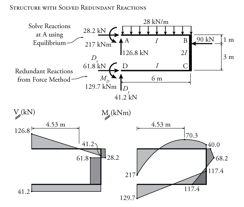
Then, knowing all of the external forces and reactions for this ${3^\circ}$ indeterminate system, we can find the final shear and moment diagrams as shown in Figure 8.22.