 Learn About Structures
If a frame does not have any translational degrees of freedom, then a slope-deflection analysis for the frame is the same as it would be for a beam. A frame that only has rotational degrees-of-freedom (no translational degrees-of-freedom) is called a non-sway frame. This concept was previously described in Figure 9.2.
Recall again the slope deflection equations from Section 9.3.
\begin{equation} \boxed{ M_{AB} = \frac{2EI}{L} (2 \theta_A + \theta_B - 3 \psi ) + \text{FEM}_{AB} } \label{eq:SD-AB} \tag{1} \end{equation} \begin{equation} \boxed{ M_{BA} = \frac{2EI}{L} (\theta_A + 2 \theta_B - 3 \psi ) + \text{FEM}_{BA} } \label{eq:SD-BA} \tag{2} \end{equation} \begin{equation} \boxed{ M_{nf} = \frac{2EI}{L} (2 \theta_n + \theta_f - 3 \psi ) + \text{FEM}_{nf} } \label{eq:SD-NF} \tag{3} \end{equation} \begin{equation} \boxed{ M_{rh} = \frac{3EI}{L} (\theta_r - \psi ) + \left( \text{FEM}_{rh} - \frac{\text{FEM}_{hr}}{2} \right) } \label{eq:SD-RH} \tag{4} \end{equation} \begin{equation} \boxed{ M_{hr} = 0 } \label{eq:SD-HR} \tag{5} \end{equation}
Example
The slope-deflection method for a non-sway frame will be illustrated using the example in Figure 9.12. In this frame, nodes C, D and E are restrained from translating horizontally by the fixed end support at node B (recall that we are considering all members to be axially rigid). The vertical translation of node C is restrained by member AC connected to the fixed end at point A, and the vertical translation of node D is restrained by the roller support at node D.
Node E shown in Figure 9.12 is able to translate vertically and rotate; however, we will see that for a free end like member DE, we can neglect the degrees-of-freedom associated with free node E by considering that the member with the free end simply contributes an equivalent point moment to member CD at node D.
Node A in Figure 9.12 experiences a support settlement of $10\mathrm{\,mm}$ downwards. Since we consider member AC to be axially rigid, this will also cause node C to move downwards by exactly $10\mathrm{\,mm}$. This settlement is not considered a degree-of-freedom since it is not free to take any value based on loading. No matter what the loading condition is on the frame, the settlement only has one set value (in this case, $10\mathrm{\,mm}$).
The frame structure in Figure 9.12 is loaded with a uniform distributed moment between nodes C and E, and a point moment at node C (positive because it is counter-clockwise). Both the Young's Modulus and moment of inertia for all frame sections are also provided in the figure.
Since we are not counting the degrees-of-freedom associated with the free end at node E, this frame structure has only two degrees of freedom total, $\theta_C$ and $\theta_D$. This makes it a good candidate for the slope-deflection method. If we wanted to do this problem with the force method, it would have 4 degrees of indeterminacy and, therefore, a systems of four equations and four unknowns to solve.
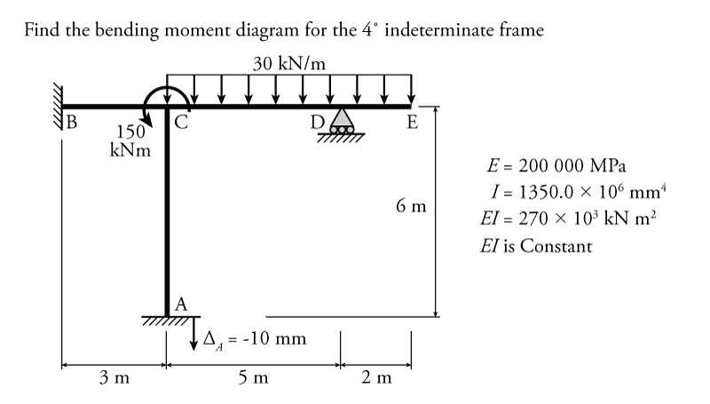
The next step in the analysis is to find an equilibrium equation for each degree-of-freedom. For this problem, the moment equilibrium for nodes C and D are shown in Figure 9.13. At node C there are three different members that frame into it, members CA, CB and CD. Each of these members has an unknown end moment $M_{CA}$, $M_{CB}$ and $M_{CD}$ as shown in the figure. These unknown moments are considered to be positive at the member ends (counter-clockwise). The moments caused by each of these members on node C itself are also shown. Since the members here are cut just beside the node, the moments on the node itself will have an equal magnitude but opposite direction to the moments at the member ends ($-M_{CA}$, $-M_{CB}$ and $-M_{CD}$ as shown in the figure). In addition to these moments that the member ends apply to the node, node C also has a clockwise point moment applied directly to it of $+150\mathrm{\,kNm}$. This point moment is also shown in the figure.
So, the left side of Figure 9.13 shows all of the moments that are applied to node C. We can now use these to construct an equilibrium condition for the moment around node C. We know that, since the node is not accelerating, all of the moments applied to it must add to zero:
\begin{align*} -M_{CA}-M_{CB}-M_{CD}+150 = 0 \end{align*}
Rearranging this:
\begin{align*} M_{CA}+M_{CB}+M_{CD} = 150\mathrm{\,kNm} \end{align*}
This is our first equilibrium condition for the slope-deflection method analysis.
The equilibrium for node D (associated with the second degree-of-freedom $\theta_D$) is shown on the right side of Figure 9.13. The member to the right of node D (member DE) has a free end at point E, as previously discussed. This free end acts like a cantilever with its root at point D. The effect of this cantilever on the moment equilibrium at node D is indistinguishable from the effect of a point moment with the same magnitude as the moment caused by the cantilever. This is because member DE with the free end does not contribute any rotational stiffness to node D, so the moment applied by member DE is independent of the amount of rotation of node D. So, member DE may be removed from our analysis and replaced by a point moment at node D that has a magnitude equal to the moment applied by member DE onto node D (as shown on the lower right of Figure 9.13).
Looking now at the moment equilibrium around node D (as shown in Figure 9.13, we get:
\begin{align*} -M_{DC} - 60 &= 0 \\ M_{DC} &= -60\mathrm{\,kNm} \end{align*}
Having developed our equilibrium conditions for nodes C and D, we can now use the slope-deflection equations to find expressions for each moment from each equilibrium condition in terms of the unknown DOFs (the rotations $\theta_{C}$ and $\theta_{D}$). Therefore, we need expressions for $M_{CB}$, $M_{CA}$, $M_{CD}$, and $M_{DC}$. Later, to find the final reaction moments at nodes A and B, we will also have to find expressions for $M_{AC}$ and $M_{BC}$. So, it makes sense to find them all at the beginning of the problem.
All of the members have either a fixed end or continuous ends at both nodes (i.e. none of the members have a pin at one end with only one member framing into it). Therefore we will use the slope deflection equation from equation \eqref{eq:SD-NF}. Member CD should not be considered to have a pinned end at node D (even though we are effectively removing member DE from our analysis), so, we cannot use equation \eqref{eq:SD-RH} for member CD. This is because member CD has a point moment at node D, and equation \eqref{eq:SD-RH} can only be used if the moment at the pinned end is equal to zero.
To find all of the end moments using the slope-deflection equations, we first need to calculate the chord rotations and the fixed end moments for each member (if they exist). In a non-sway frame, chord rotations will only be caused by support settlements or other support movements. In this example, there is a support settlement of node A by $10\mathrm{\,mm}$ downwards (as shown in Figure 9.14). When node A displaces downwards, this also causes node C to displace downwards by an equal amount ($10\mathrm{\,mm}$) because we are considering all members to be axially rigid. This causes the element chords of members BC and CD to rotate to accommodate that downwards displacement. Recall that the element chord is simply a straight line drawn between the two element end nodes as shown in the figure.
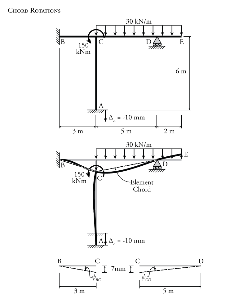
The rotation for each chord may be calculated as shown in Figure 9.14. For member BC, the chord rotation is:
\begin{align*} \psi_{BC} &= \frac{\Delta}{L} \\ \psi_{BC} &= \frac{-10}{3000} \\ \psi_{BC} &= -0.00333\mathrm{\,rad} \curvearrowright \end{align*}
The chord rotation for member BC is negative because the chord rotates clockwise from its initial position as point C settles downwards. Likewise, for member CD:
\begin{align*} \psi_{CD} &= \frac{-10}{-5000} \\ \psi_{CD} &= +0.00200\mathrm{\,rad} \curvearrowleft \end{align*}
The chord rotation for member CD is positive because the chord rotates counter-clockwise from its initial position as point C settles downwards. There is only one chord rotation for each member. Regardless of which end node is considered as the centre of rotation, the rotation direction for a member will be the same.
Member DE would also have some chord rotation, but since we are replacing member DE by an equivalent point moment at node D (as discussed previously), then we do not have to consider the behaviour of member DE explicitly at this point.
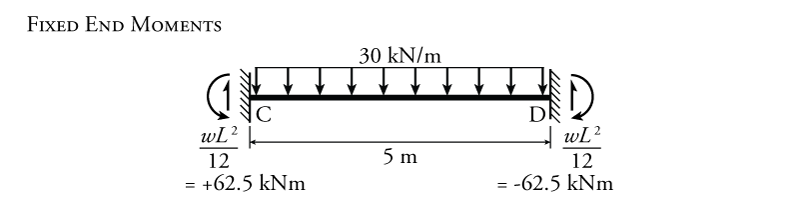
Fixed end moments are required for each member that has loads applied to the member between the end nodes. In our example, only member CD will have fixed end moments. The effect of the distributed load on member DE has already been converted to an effective point moment at point D in the equilibrium equation. The calculation of the fixed end moments for member CD are shown in Figure 9.15. The values for the fixed end moments in the figure are taken from the previous Figure 9.6. Since we are considering counter-clockwise moments to be positive and clockwise moments to be negative, the moment at node C is positive an the moment at point D is negative as shown in the figure. This gives us:
\begin{align*} \text{FEM}_{CD} &= +62.5\mathrm{\,kNm} \curvearrowleft \\ \text{FEM}_{DC} &= -62.5\mathrm{\,kNm} \curvearrowright \end{align*}
Since member CD is the only member with external loads between the nodes:
\begin{align*} \text{FEM}_{AC} = \text{FEM}_{CA} = \text{FEM}_{BC} = \text{FEM}_{CB} = 0 \end{align*}
Now that we have found all of the chord rotations and fixed end forces for all members, we can use the slope deflection equation \eqref{eq:SD-NF} to find the end moments for each member in terms of the end rotations. For $M_{AC}$:
\begin{align*} M_{nf} &= \frac{2EI}{L} (2 \theta_n + \theta_f - 3 \psi ) + \text{FEM}_{nf} \end{align*}
For the moment at the end of member AC at point A, A is the near side and C is the far side, so:
\begin{align*} M_{AC} &= \frac{2EI}{L} (2 \theta_A + \theta_C - 3 \psi_{AC} ) + \text{FEM}_{AC} \\ M_{AC} &= \frac{2EI}{6} (2 \theta_A + \theta_C - 3 (0) ) + 0 \end{align*}
Since node A is fixed, we know that $\theta_A =0$, so:
\begin{equation*} \boxed{M_{AC} = \frac{2EI}{6} (\theta_C) = 0.333 EI \theta_C } \end{equation*}
For $M_{CA}$:
\begin{align*} M_{CA} &= \frac{2EI}{L} (2 \theta_C + \theta_A - 3 \psi_{AC} ) + \text{FEM}_{CA} \\ M_{CA} &= \frac{2EI}{6} (2 \theta_C + \theta_A - 3 (0) ) + 0 \end{align*}
Again, since node A is fixed, we know that $\theta_A =0$, so:
\begin{equation*} \boxed{M_{CA} = 0.667 EI \theta_C } \end{equation*}
For $M_{BC}$:
\begin{align*} M_{BC} &= \frac{2EI}{L} (2 \theta_B + \theta_C - 3 \psi_{BC} ) + \text{FEM}_{BC} \\ M_{BC} &= \frac{2EI}{3} (2 \theta_B + \theta_C - 3 (-0.00333) ) \end{align*}
Since node B is fixed, then we know that $\theta_B =0$, so:
\begin{align*} M_{BC} &= \frac{2EI}{3} ( \theta_C + 0.0100 ) \\ M_{BC} &= 0.667EI\theta_C + 0.00667 EI \end{align*}
Substituting in $EI = 270\times 10^3\mathrm{\,kN m^2}$ (see Figure 9.12):
\begin{equation*} \boxed{M_{BC} = 0.667 EI \theta_C + 1800.9 } \end{equation*}
For $M_{CB}$:
\begin{align*} M_{CB} &= \frac{2EI}{L} (2 \theta_C + \theta_B - 3 \psi_{BC} ) + \text{FEM}_{CB} \\ M_{CB} &= \frac{2EI}{3} (2 \theta_C + \theta_B - 3 (-0.00333) ) \end{align*}
Since node B is fixed, then we know that $\theta_B =0$, so:
\begin{align*} M_{CB} &= \frac{2EI}{3} ( 2 \theta_C + 0.0100 ) \\ M_{CB} &= 1.333EI\theta_C + 0.00667 EI \end{align*} \begin{equation*} \boxed{M_{CB} = 1.333 EI \theta_C + 1800.9 } \end{equation*}
For $M_{CD}$:
\begin{align*} M_{CD} &= \frac{2EI}{L} (2 \theta_C + \theta_D - 3 \psi_{CD} ) + \text{FEM}_{CD} \\ M_{CD} &= \frac{2EI}{5} (2 \theta_C + \theta_D - 3 (0.00200) ) + 62.5 \end{align*} \begin{equation*} \boxed{M_{CD} = 0.8 EI \theta_C + 0.4 EI \theta_D - 585.5 } \end{equation*}
For $M_{DC}$:
\begin{align*} M_{DC} &= \frac{2EI}{L} (2 \theta_D + \theta_C - 3 \psi_{CD} ) + \text{FEM}_{DC} \\ M_{DC} &= \frac{2EI}{5} (2 \theta_D + \theta_C - 3 (0.00200) ) - 62.5 \end{align*} \begin{equation*} \boxed{M_{DC} = 0.8 EI \theta_D + 0.4 EI \theta_C - 710.5 } \end{equation*}
These six equations represent the moment at each end of every member in the structure in terms of the unknown DOF rotations $\theta_C$ and $\theta_D$ only. We can now take these end moment expressions and substitute them back into the equilibrium conditions to solve for $\theta_C$ and $\theta_D$. The first equilibrium equation:
\begin{align*} M_{CA}+M_{CB}+M_{CD} &= 150 \\ [0.667 EI \theta_C] + [1.333 EI \theta_C + 1800.9] + [0.8 EI \theta_C + 0.4 EI \theta_D - 585.5] & = 150 \\ 2.80 EI \theta_C + 0.4 EI \theta_D + 1065.4 &= 0 \end{align*}
and the second equilibrium equation:
\begin{align*} M_{DC} &= -60 \\ 0.8 EI \theta_D + 0.4 EI \theta_C - 710.5 &= -60 \\ 0.8 EI \theta_D + 0.4 EI \theta_C - 650.5 &= 0 \\ \theta_C &= \frac{650.5 - 0.8 EI \theta_D}{0.4EI} \end{align*}
Substitute this expression for $\theta_C$ back into the first equilibrium equation:
\begin{align*} 2.8 EI \left( \frac{650.5 - 0.8 EI \theta_D}{0.4EI} \right) + 0.4 EI \theta_D + 1065.4 &= 0 \\ 4553.5 - 5.6EI \theta_D + 0.4EI \theta_D + 1065.4 &= 0 \\ \theta_D &= \frac{5618.9}{5.2EI} \end{align*} \begin{equation*} \boxed{ \theta_D = \frac{1080.6}{EI} = +0.00400\mathrm{\,rad} \curvearrowleft} \end{equation*}
Therefore,
\begin{align*} \theta_C &= \frac{650.5 - 0.8 EI \left( \frac{1080.6}{EI} \right)}{0.4EI} \end{align*} \begin{equation*} \boxed{ \theta_C = -\frac{535.0}{EI} = -0.00198\mathrm{\,rad} \curvearrowright} \end{equation*}
These rotations are the solutions to the unknown rotational degrees-of-freedom that were identified at the beginning of the problem.
Knowing these rotations, we can substitute $\theta_C$ and $\theta_D$ back into the end moment equations that we previously constructed using the slope-deflection equation. This gives us actual values for the magnitudes and directions of the end moments for all of the members:
\begin{align*} M_{AC} &= -178.2\mathrm{\,kNm} \curvearrowright \\ M_{CA} &= -356\mathrm{\,kNm} \curvearrowright \\ M_{BC} &= +1444\mathrm{\,kNm} \curvearrowleft \\ M_{CB} &= +1088\mathrm{\,kNm} \curvearrowleft \\ M_{CD} &= -581\mathrm{\,kNm} \curvearrowright \\ M_{DC} &= -60\mathrm{\,kNm} \curvearrowright \end{align*}
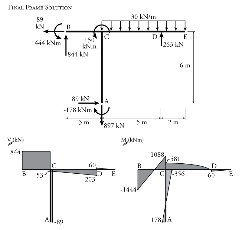
Using equilibrium on individual members as shown in Figure 9.16, the shears forces at the ends of each member may be found based on the known end moments. For example, for member BC, the shear at the left end ($V_{BC}$) may be found by evaluating the moment equilibrium around node C (making sure to include both end moments and the moment effect caused by the external loads between nodes B and C). The axial forces for each member may then be calculated using the member end shear forces. Examples for the calculation of axial forces in members BC and AC are shown in the figure.
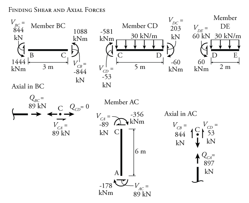
Axial forces and shear forces at support locations can then be used to find the reaction forces. The complete resulting free body diagram for the entire frame is shown in Figure 9.17. The individual member free body diagrams from Figure 9.16 may also be used to draw shear and moment diagrams for the structure. The resulting shear and moment diagrams for this example structure are shown in Figure 9.17.