 Learn About Structures
Now that we know how to construct influence lines, how do we use them, and what are they good for? The biggest benefit is that once you construct an influence line for a reaction, shear or moment at a critical location in a structure, you can easily check how multiple different load patterns on the structure will affect that load effect (the reaction, shear or moment). For example, if we are designing the reaction base for a beam, we can first construct the influence line for that reaction. Then, we can use that influence line to check multiple different load patterns and load cases on the beam without having to re-analyse the beam for every different set of loads. This is particularly useful if you have to check multiple different load patterns to find the worst possible combination, or if you have a moving load caused by a vehicle.
In this section, we will look at three main applications for influence lines. The first is the use of an influence line to determine the influence of a single point load. The second is the use of an influence line to determine the effect of a distributed load or patterned distributed load. The last is the use of an influence line to determine the effect of a moving pattern of loads.
The Influence of a Point Load
Up to now, we have only seen how influence lines show us the effect of a unit point load moving along a beam (with a magnitude of 1.0); however, an influence line may be used to determine the effect of any magnitude point load on a beam. All we have to do is multiply the magnitude of the applied point load by the value of the influence line at the location where the point load is applied.
For example, a sample influence line for a vertical support reaction $C_y$ is shown at the top of Figure 6.16 (IL $C_y$). If we apply a point load of $13\mathrm{\,kN}$ at point E, as shown, then the reaction force $C_y$ will be equal to:
\begin{align*} C_y &= 13\mathrm{\,kN}(-0.4)= - 5.2\mathrm{\,kN} \\ &= 5.2\mathrm{\,kN} \downarrow \end{align*}
where $0.4$ is the value of the influence line at point E as shown.
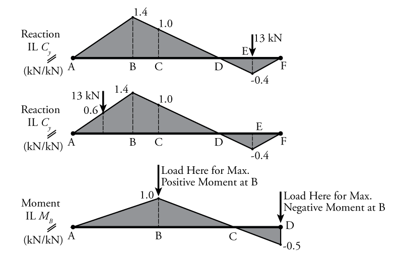
Likewise, if you were to put that point load anywhere else along the beam, the effect on $C_y$ would be equal to the value of the point load multiplied by the value of the influence line at that location. Another example is shown in the middle diagram in Figure 6.16. Here an in-between influence line value at a point between A and B is found using similar triangles to be equal to 0.6. If the $13\mathrm{\,kN}$ point load is applied at this location, then the reaction $C_y = 13(0.6) = 7.8\mathrm{\,kN} \uparrow$.
In addition to telling us what the effect of a certain load will be on a parameter such as the reaction at a certain point, the influence line also gives us a visual indication of where a load should be placed to create the maximum positive or negative effect. For example, the bottom diagram in Figure 6.16 shows an influence diagram for some internal moment in a beam $M_B$. From this diagram, it is clear that if a load may be placed anywhere along the beam, then placing the load at point B would cause the greatest positive internal moment at point B ($M_B$) and placing the load at point D would cause the maximum negative moment at point B ($M_B$).
The Influence of a Distributed Load
Influence lines also allow us to easily find the effect of distributed loads on individual response parameters (e.g. reactions, shear at a point). To do this, we simply find the area underneath the influence diagram for the parts of the diagram where a uniform distributed load is applied and then multiply that area by the magnitude of the uniform load.
An example of this is shown in Figure 6.17. At the top of this figure, an influence diagram is shown for the vertical reaction at a point C (IL $C_y$). If a $16\mathrm{\,kN/m}$ distributed load is applied between points B and C, the we can find the effect of the distributed load on the reaction $C_y$ by multiplying the area under the influence diagram in the applied load location (the trapezoidal area shaded in the figure) by the value of the distributed load ($16\mathrm{\,kN/m}$):
\begin{align*} C_y &= \frac{1.4+1.0}{2}(4\mathrm{\,m})(16\mathrm{\,kN/m}) \\ C_y &= 76.8\mathrm{\,kN} \uparrow \end{align*}
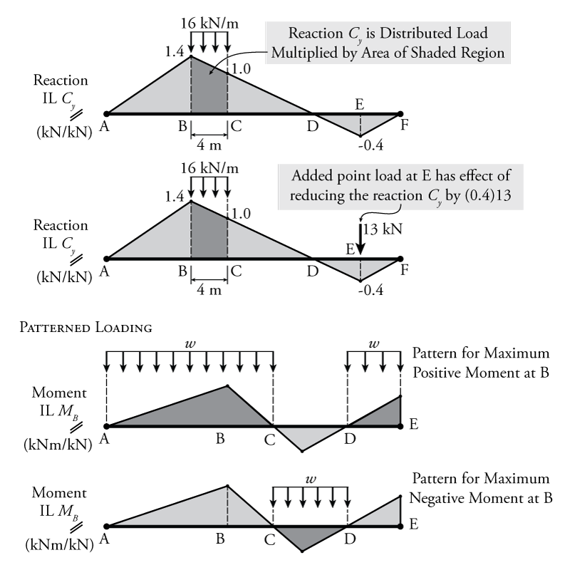
If we then added a point load to the beam simultaneously as shown in the second diagram in Figure 6.17, the effect of the distributed load and point load together will be additive:
\begin{align*} C_y &= \frac{1.4+1.0}{2}(4\mathrm{\,m})(16\mathrm{\,kN/m}) + 13\mathrm{\,kN}(-0.4) \\ C_y &= 71.6\mathrm{\,kN} \uparrow \end{align*}
Like the point load case discussed in the previous section, influence diagrams can also help us to determine where we should load the beam to cause the worst effect on a parameter. This is illustrated by the bottom two diagrams in Figure 6.17. If we would like to find the distributed loading pattern that will cause the greatest positive moment at B ($M_B$), then we should only load between points A and C and between points D and E as shown in the figure. If we were to also load the rest of the beam between C and D, then our moment would actually decrease. Patterned loading like this is a common design case in structural engineering, and this example makes it clear that sometimes considering a distributed load to act along the entire length of a beam can actually be unconservative! We could actually get worse moment by leaving some of the load off.
Likewise, if we want to find the distributed loading pattern that will cause the greatest negative moment at B, then we should only load the beam between points C and D as shown in Figure 6.17.
The Influence of a Series of Moving Loads
The effect of a series of point loads on a certain response parameter (such as a reaction or internal moment at a point) may be found by simply adding up the effect of each individual point load. But, what would happen if we have a set of point loads in a certain series and that series of loads may be placed at any point along the beam? How do we find the worst case location for the series of loads?
This is a common design problem in bridge engineering, since one of the design loads is a series of loads caused by a "standard" truck, which can move anywhere along the length of the bridge. One example of a standard set of truck loads for Ontario, Canada is shown in Figure 6.18. Since the truck has multiple wheels/axles, the total load of the truck is not spread evenly over its length, but is concentrated at the locations of the wheel axles. The standard truck shown in the figure is designed to be a worst-case heavy truck.

If we want to find the worst effect of such a set of moving loads, caused by a truck or otherwise, then we can use the influence line to easily find it. It may seem like there are an infinite number of possibilities for the location of a moving truck on a bridge, but, luckily, it can be shown that the worst case will always be when one of the loads is placed on a peak of the influence diagram. So, we only need to check the possibilities where each load is placed on a peak.
An example of this method is shown in Figure 6.19. A sample influence diagram for the shear in a beam at point B is shown at the top of the figure (IL $V_B$), and we must find the maximum positive shear that will be caused by the set of moving loads shown on the top right of the figure. This moving set of loads consists of three different loads with different magnitudes $P_1$, $P_2$, and $P_3$. The loads are spaced apart as shown and that spacing is constant.
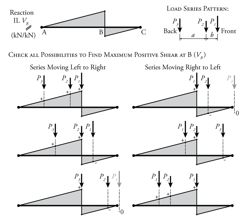
There is only one peak for the positive shear in the influence diagram, and that peak is located just immediately to the left of point B. Therefore, the worst case will occur when one of the loads $P_1$, $P_2$, or $P_3$ is located right at point B (actually just immediately to the left of point B). All of the possibilities for this are shown in Figure 6.19. Note that, since the series could potentially travel in either direction across the beam, we need to check both the cases where it moves from left to right (where the front load $P_1$ is on the right), and the cases where it moves from right to left (where the front load $P_1$ is on the left).
To find the total shear $V_B$ caused by each possibility shown in Figure 6.19, all we have to do is add up the effect of each point load (the value of the point load multiplied by the value of the influence line at the point load's location). Sometimes, one of the loads may fall off of the beam altogether, as shown in the figure. In that case, that load is ignored and not added to the others. Of course, loads that cause a negative shear effect would be subtracted from the total. At the end, whichever possibility creates the greatest possible shear at point B constitutes the worst case load series location.