 Learn About Structures
For the analysis of non-sway frames, the moment distribution method may be applied in the exact same way as for beams. The only difference is that there may be more than two elements attached to each node. Distribution factors can easily be calculated for such nodes as previously shown and discussed in Figure 10.4.
For sway frames, extra steps are required. A unit deformation must be applied to the degree-of-freedom associated with the sway, and the resulting force must be scaled to the force resulting from the full system restrained at that degree of freedom. Analysis of sway frames using the moment distribution method is not within the scope of this book.
Example
The analysis of a non-sway frame using the moment distribution method will be illustrated using the example structure shown in Figure 10.8. This structure has members of varying size (moment of inertia $I_0$ or $2I_0$) and an overhang to the right of node C. To solve this problem we will use the same method that was used for beams, as described in Section 10.3.
First, we will find the stiffness for each member using equations \eqref{eq:stiff-fix} and \eqref{eq:stiff-pin}.
\begin{equation} \boxed{ k_{AB} = \frac{4EI}{L} } \label{eq:stiff-fix} \tag{1} \end{equation} \begin{equation} \boxed{ k_{AB} = \frac{3EI}{L} } \label{eq:stiff-pin} \tag{2} \end{equation}
Member AB has a pin end at node A, so the stiffness is:
\begin{align*} k_{AB} &= \frac{3EI}{L} \\ k_{AB} &= \frac{3E(2I_0)}{5} \\ k_{AB} &= 1.2EI_0 \end{align*}
All of the rest of the members are fixed at both ends (assuming all of the nodes are originally locked for rotation), so:
\begin{align*} k_{BC} = &= \frac{4EI}{L} \\ k_{BC} &= \frac{4E(2I_0)}{4} \\ k_{BC} &= 2.0EI_0 \end{align*}
and similarly,
\begin{align*} k_{BE} &= 1.0EI_0 \\ k_{CF} &= 2.0EI_0 \end{align*}
Member CD has no stiffness associated with it since the right end at node D is free (and so has no resistance to rotation). Similarly to the slope-deflection method, we will deal with the cantilevered overhang by replacing it with an effective point moment at the root of the cantilever at node C.
Knowing the stiffness of each member, we can find all of the distribution factors for each node. Recall that each node has as many distribution factors as there are members connected to the node. Again, since node D is free, no moment can be distributed into member CD from node C (the member has no stiffness because of the free end). So,
\begin{align*} \text{DF}_{CD} = 0 \end{align*}
As discussed previously in Section 10.3, pinned supports with only one member connected have a distribution factor of 1.0 and fixed supports have a distribution factor of 0, so:
\begin{align*} \text{DF}_{AB} &= 1.0 \\ \text{DF}_{EB} &= 0.0 \\ \text{DF}_{FC} &= 0.0 \end{align*}
Recall that the notation $\text{DF}_{AB}$ means the distribution factor for member AB at node A. Likewise, $\text{DF}_{BA}$ would be the distribution factor for member AB at node B.
The remainder of the distribution factor are calculated based on the relative stiffness of all of the members framing into a joint (as previously shown in Figure 10.4). At node B:
\begin{align*} \text{DF}_{BA} &= \frac{k_{AB}}{k_{AB}+k_{BC}+k_{BE}} \\ \text{DF}_{BA} &= \frac{1.2EI_0}{1.2EI_0+2.0EI_0+1.0EI_0} \\ \text{DF}_{BA} &= 0.286 \end{align*} \begin{align*} \text{DF}_{BC} &= \frac{k_{BC}}{k_{AB}+k_{BC}+k_{BE}} \\ \text{DF}_{BC} &= \frac{2.0EI_0}{1.2EI_0+2.0EI_0+1.0EI_0} \\ \text{DF}_{BC} &= 0.476 \end{align*} \begin{align*} \text{DF}_{BE} &= \frac{k_{BE}}{k_{AB}+k_{BC}+k_{BE}} \\ \text{DF}_{BE} &= \frac{1.0EI_0}{1.2EI_0+2.0EI_0+1.0EI_0} \\ \text{DF}_{BE} &= 0.238 \end{align*}
Notice that all of these distribution factors at node B must add up to 1.0:
\begin{align*} \text{DF}_{BA} + \text{DF}_{BC} + \text{DF}_{BE} = 1.0 \end{align*}
At node C:
\begin{align*} \text{DF}_{CB} &= \frac{k_{BC}}{k_{BC}+k_{CD}+k_{CF}} \\ \text{DF}_{CB} &= \frac{2.0EI_0}{2.0EI_0+0+2.0EI_0} \\ \text{DF}_{CB} &= 0.500 \end{align*} \begin{align*} \text{DF}_{CF} &= \frac{k_{CF}}{k_{BC}+k_{CD}+k_{CF}} \\ \text{DF}_{CF} &= \frac{2.0EI_0}{2.0EI_0+0+2.0EI_0} \\ \text{DF}_{CF} &= 0.500 \end{align*}
Notice that, although there is only one stiffness term for each member, the distribution factors at two ends of a member a not likely to be the same. In this case, $\text{DF}_{BC} = 0.476$ is not equal to $\text{DF}_{CB} = 0.500$. These are different because they depend on the other members that connect to the same node.
The last step before conducting the moment distribution process with the table is to find the fixed end moments for each member. These fixed end moments give us the starting condition moments in our frame (before we start unlocking any nodes to allow them to rotate into equilibrium). To find these, we can use Figure 9.6 as shown in Figure 10.9.
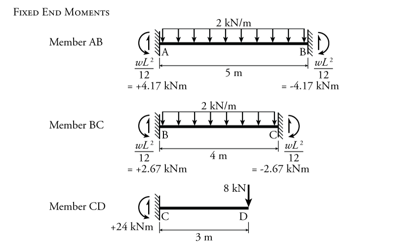
In this case, members AB and BC have uniformly distributed loads that result in fixed end moments equal to $\frac{wL^2}{12}$ at either end as shown in Figure 10.9. We must be careful to use the correct sign for these moments in our analysis. Recall that counter-clockwise moments are considered positive, and clockwise moments are considered negative as per our sign convention. So,
\begin{align*} \text{FEM}_{AB} &= \frac{wL^2}{12} \\ \text{FEM}_{AB} &= \frac{2(5)^2}{12} \\ \text{FEM}_{AB} &= +4.17\mathrm{\,kNm}\; (\curvearrowleft) \\ \text{FEM}_{BA} &= -4.17\mathrm{\,kNm}\; (\curvearrowright) \end{align*}
Likewise:
\begin{align*} \text{FEM}_{BC} &= \frac{wL^2}{12} \\ \text{FEM}_{BC} &= \frac{2(4)^2}{12} \\ \text{FEM}_{BC} &= +2.67\mathrm{\,kNm}\; (\curvearrowleft) \\ \text{FEM}_{CB} &= -2.67\mathrm{\,kNm}\; (\curvearrowright) \end{align*}
Lastly, we will consider the overhang CD to contribute a fixed end moment at node C (caused by the load at the end of the cantilever at node D). This fixed end moment is simply equal to the moment at the root of the cantilever at point C as shown in the lower diagram of Figure 10.9:
\begin{align*} \text{FEM}_{CD} &= 8(3) \\ \text{FEM}_{CD} &= 24.0\mathrm{\,kNm} (\curvearrowleft) \end{align*}
We must be careful with the sign of this moment. To be consistent with the other fixed end moments, this moment must be the end moment at the end of member CD at point C, as shown in the figure, not the moment that is applied to node C. The end moment on member CD at point C is counter-clockwise as shown in the figure, so $\text{FEM}_{CD}$ must be positive.
We now have all of the input parameters that are necessary to solve the moment distribution analysis. The moment distribution analysis is shown in Table 10.2.
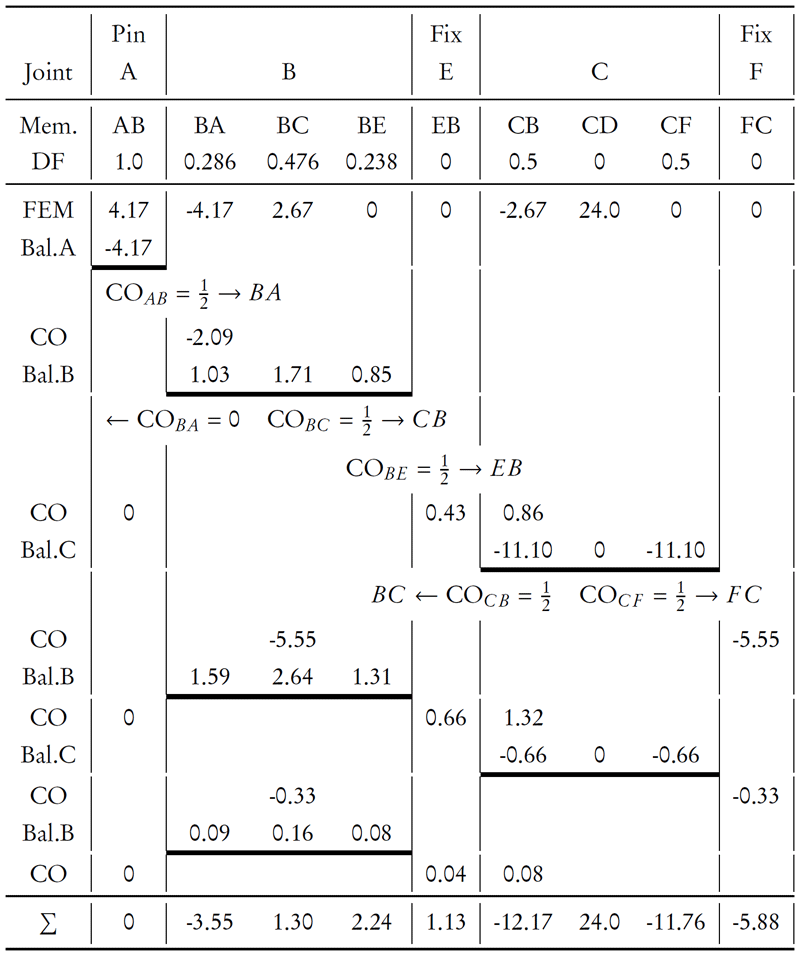
As before, the moment distribution analysis in Table 10.2 starts with the application of the fixed end moments for each member (with the correct sign used as discussed previously). We can start with any node, but often it makes sense to balance out the pinned nodes first. We cannot carry-over any moments into a pin, once we balance a pin node once, we do not have to visit it again. Recall as well that we do not balance fixed support nodes. Since their distribution factor is zero, any moment that is applied or carried over to a fixed end will stay there for the duration of the analysis. This makes sense because we cannot release a fixed support to allow it to adjust into equilibrium. A fixed support is already in equilibrium (the end moment from the members is balanced by the reaction moment provided by the fixed support).
So, we start by balancing the moments at the pinned support at node A as shown in Table 10.2. Since there is only one moment provided by member AB, we simply apply the reverse moment to bring the node into equilibrium ($-4.17\mathrm{\,kNm}$). The think line below this balancing moment in the table at node A signifies that all of the moments above that line for node A are in equilibrium (they all add up to zero). Next, we must carry-over half of that balancing moment to the other end of the member BA ($-2.09\mathrm{\,kNm}$). This carry over moment has the same sign as the balancing moment.
After we are done with the pin node A, we can move on to one of the other nodes that must be balanced. We have an option of either node B or node C (nodes E and F have fixed supports). For this example, we will proceed with balancing node B as shown in Table 10.2. To balance this node, we must first sum up all of the previous unbalanced moments that have been applied to that node (due to fixed end moments or previous carry-overs). We get:
\begin{align*} \sum M_B = -4.17 + 2.67 - 2.09 = -3.59 \end{align*}
Then, we need to distribute the reverse of that unbalanced moment ($+3.59$) to all three members connected to that node based on their relative stiffness. We do this using the distribution factors, which we previously calculated and are shown at the top of the table. For example, for member BA, we multiply the balancing moment $+3.59$ by the distribution factor for BA which is $\text{DF}_{BA} = 0.286$ to get $1.03$. We repeat this calculation with the other two members at node B to get the other balancing moments shown in the table. Again, once the node is in equilibrium, we can draw a horizontal line below the balancing moments to indicate this. Next, we must carry these moments over to the opposite ends of the member as necessary. For BA, the other end is a pin with only the one member connected to it, so we do not carry-over any moment (because the pin cannot resist any moment). For BC, we must carry-over half of the moment to the other end of the member (CB) and the same for BE, which has half carried-over to EB as shown.
Once we have finished the carry-over step, we can move onto the next node. At this point we only have one node with unbalanced moments, node C. So, we find the total unbalanced moment on node C:
\begin{align*} \sum M_C = -2.67 + 24 + 0.86 = +22.19 \end{align*}
and apply the reverse of that total unbalanced moment to each member end using the distribution factors again as shown in Table 10.2. This time, we have two carry-overs, one from CB to BC and one from CF to FC.
The carry-over to BC from node C, disturbs the equilibrium that was achieved for node B in the previous step. So, we must rebalance node B as shown in Table 10.2 to account for this new carry-over moment of $-5.55$ at member end BC. Note that we only have to consider this new moment, all of the moments above the previous horizontal line for node B are already in equilibrium, adding up to zero. So, we apply the inverse of $-5.55$ ($+5.55$) and again distribute it to all of the members connected to point B using the distribution factors. Then, we carry-over to the opposite ends of all the members again. The carry-over from BC to CB disturbs the moment equilibrium at node C.
So, we need to balance node C again as shown in Table 10.2. Every time we balance node B, we disturb the equilibrium at node C. Likewise, Every time we balance node C, we disturb the equilibrium at node B. This is an endless cycle; however, each time we perform this balancing by releasing the node at allowing it to move into equilibrium, the carry-over moments get smaller and smaller. By the time we get to the third balancing of node B (as shown in the table), the carry-over moments are on the order of $0.08\mathrm{\,kN}$. This is on the order of 0.3% to 2% of the initial fixed end moments. What is left to balance at this point can be considered error in our analysis. If we continue to do more iterations, we can get as small of an error as we would like.
If I consider the current level of error to be small enough, I can finish the analysis by summing all of the columns in the table (including the initial fixed end moments) to get the total end moment for each end of each member (as shown in the bottom row of Table 10.2). Pinned ends (such as node A) will have a total moment of zero. Member ends at fixed support location (such as nodes E and F) will have non-zero total end moments which are in equilibrium with the moment reactions at the fixed supports. For other nodes (such as nodes B and C), the sum of all the final end moments for the connected members must be zero (within the margin of error of the analysis). This is the case for the end moments shown in Table 10.2. If this is not the case, then there must be some error in the analysis.
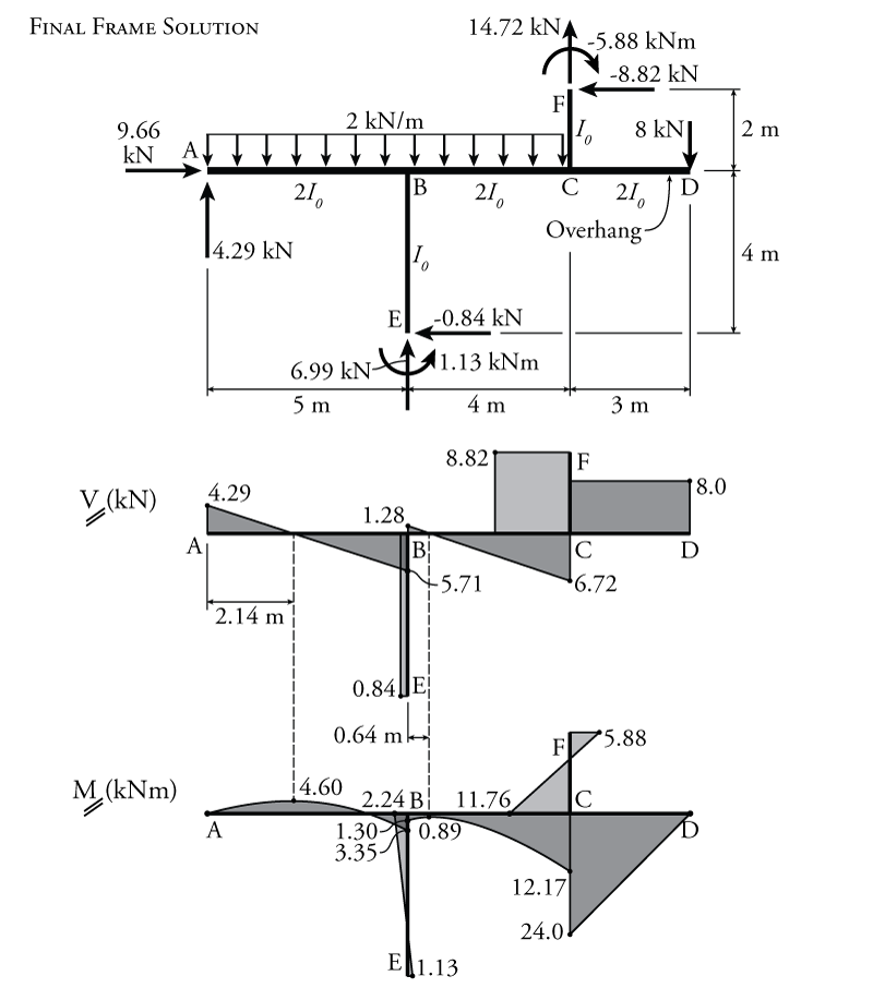
Once we have finished the iterative part of the moment distribution method analysis, we can use the end moments to calculate the shears and axial forces in each member of the frame as shown in Figure 10.10. This is the same as what was done previously in the slope deflection method analyses (see Chapter 9).
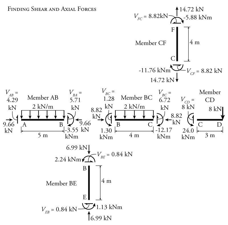
Then, knowing the shears and end moments, the shear and moment diagrams for the frame may be constructed as shown in Figure 10.11.