>>When you're done reading this section, check your understanding with the interactive quiz at the bottom of the page.

The method of joints is a procedure for finding the internal axial forces in the members of a truss. It involves a progression through each of the joints of the truss in turn, each time using equilibrium at a single joint to find the unknown axial forces in the members connected to that joint.

To perform a 2D truss analysis using the method of joints, follow these steps:

1. Check that the truss is determinate and stable using the methods from Chapter 2.
2. If possible, reduce the number of unknown forces by identifying any zero force members in the truss.
3. Calculate the support reactions for the truss using equilibrium methods as discussed in Section 3.4
4. Identify a starting joint that has two or fewer members for which the axial forces are unknown.
5. Draw a free body diagram of the joint and use equilibrium equations to find the unknown forces.
6. Move on to another joint that has two or fewer members for which the axial forces are unknown. Solve the unknown forces at that joint. Continue through the structure until all of the unknown truss member forces are known.

If the truss is determinate and stable there will always be a joint that has two or fewer unknowns. The critical number of unknowns is two because at a truss joint, we only have the two useful equilibrium equations \eqref{eq:TrussEquil}.

\begin{equation}\label{eq:TrussEquil}\tag{1} \sum_{i=1}^{n}{F_{xi}} = 0; \sum_{i=1}^{p}{F_{yi}} = 0; \end{equation}

Example - Method of Joints

Figure 3.5: Method of Joints Example Problem

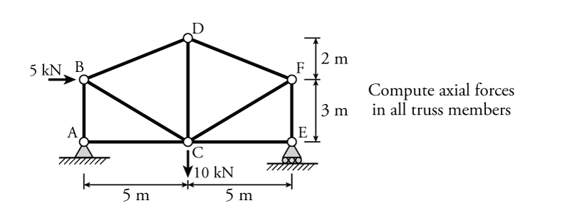
The truss shown in Figure 3.5 has external forces and boundary conditions provided. Find the internal axial forces in all of the truss members.

1. Check determinacy and stability

   This is a simple truss that is simply supported (with pin at one end and a roller at the other). From Section 2.5:

   \begin{align*} m+r &= 2j \text{ for determinacy} \\ m+r &= 9 + 3 = 12 \\ 2j &= 2(6) = 12 \end{align*}

   Therefore, the truss is determinate. There is also no internal instability, and therefore the truss is stable.

2. Identify zero force members

   Although there are no zero force members that can be identified direction using Case 1 or 2 in Section 3.3, there is a zero force member that may still easily be identified. Since the boundary support at point E is a roller, there is no horizontal reaction. Therefore, the reaction at E is purely vertical. Therefore the only horizontal force at the joint can come from member CE, but since there is not any other member or support to resist such a horizontal force, we must conclude that the force in member CE must be zero:

   \begin{equation*} \boxed{ F_{CE} = 0 } \end{equation*}

   Like any zero force member, if we did not identify the zero force member at this stage, we would be able to find it easily through the analysis of the FBDs at each joint. Finding it now just has the benefit of saving us work later.

   Note also that although member CE does not have any axial load, it is still required to exist in place for the truss to be stable. If member CE were removed, joint E would be completely free to move in the horizontal direction, which would lead to collapse of the truss.

3. Find the support reactions using global equilibrium

   Figure 3.6 shows the truss system as a free body diagram and labels the inclination angles for all of the truss members. All supports are removed and replaced by the appropriate unknown reaction force components.

   

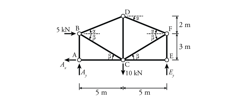   Figure 3.6: Method of Joints Example - Global Free Body Diagram

   The inclination angles $\alpha$ and $\beta$ may be found using trigonometry (equation \eqref{eq:incl-angle}):

   \begin{equation} \theta = \arctan \left( \frac{L_y}{L_x} \right) \label{eq:incl-angle} \tag{2} \end{equation} \begin{align*} \alpha &= \tan^{-1} \left( \frac{2}{5} \right) = {21.8^\circ} \\ \beta &= \tan^{-1} \left( \frac{3}{5} \right) = {31.0^\circ} \end{align*}

   The unknown reaction forces $A_x$, $A_y$ and $E_y$ can then be found using the three global equilibrium equations in 2D. Like previously, we will start with moment equilibrium around point A since the unknown reactions $A_x$ and $A_y$ both push or pull directly on point A, meaning neither of them create a moment around A. The only remaining unknown for the moment equilibrium around A will be $E_y$:

   \begin{align*} \curvearrowleft \sum M_A &= 0 \\ - 5\mathrm{\,kN} ( 3\mathrm{\,m} ) &- 10\mathrm{\,kN} ( 5\mathrm{\,m} ) + E_y ( 10\mathrm{\,m} ) = 0 \\ E_y &= +6.5\mathrm{\,kN} \end{align*} \begin{equation*} \boxed{E_y = 6.5\mathrm{\,kN} \uparrow} \end{equation*}

   We have assumed in Figure 3.6 that the unknown reaction $E_y$ points upward. Since the resulting value for $E_y$ was positive, we know that this assumption was correct, and hence that the reaction $E_y$ points upward.

   Next, consider vertical equilibrium:

   \begin{align*} \uparrow\sum F_y &= 0 \\ A_y - 10\mathrm{\,kN} + E_y &= 0 \\ A_y - 10\mathrm{\,kN} + 6.5\mathrm{\,kN} &= 0 \\ A_y &= +3.5\mathrm{\,kN} \end{align*} \begin{equation*} \boxed{A_y = 3.5\mathrm{\,kN} \uparrow} \end{equation*}

   The positive result for $A_y$ indicates that $A_y$ points upwards.

   For horizontal equilibrium, there is only one unknown, $A_x$:

   \begin{align*} \rightarrow\sum F_x &= 0 \\ -A_x + 5.0\mathrm{\,kN} &= 0 \\ A_x &= +5.0\mathrm{\,kN} \end{align*} \begin{equation*} \boxed{A_x = 5.0\mathrm{\,kN} \leftarrow} \end{equation*}

   For the unknown reaction $A_x$, we originally assumed that it pointed to the left, since it was clear that it had to balance the external $5\mathrm{\,kN}$ force.

4. Identify a starting joint

   We will select joint A as the starting joint. Since we have already determined the reactions $A_x$ and $A_y$ using global equilibrium, the joint has only two unknowns, the forces in members AB ($F_{AB}$) and AC ($F_{AC}$).

   Alternatively, joint E would also be an appropriate starting point.

5. Find the unknown forces at the starting joint

   A free body diagram of the starting joint (joint A) is shown at the upper left of Figure 3.7. The reactions $A_x$ and $A_y$ are drawn in the directions we know them to point in based on the reactions that we previously calculated.

   

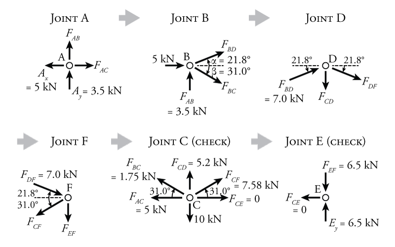   Figure 3.7: Method of Joints Example - Joint Free Body Diagrams

   The unknown member forces $F_{AB}$ and $F_{AC}$ are assumed to be in tension (pulling away from the joint). As discussed previously, there are two equilibrium equations for each joint ($\sum F_x = 0$ and $\sum F_y = 0$). Since we have two equations and two unknowns, we can solve for the unknowns easily. Horizontal equilibrium:

   \begin{align*} \rightarrow \sum F_x &= 0 \\ -A_x + F_{AC} &= 0 \\ -5\mathrm{\,kN} + F_{AC} &= 0 \\ F_{AC} &= +5\mathrm{\,kN} \end{align*} \begin{equation*} \boxed{F_{AC} = 5\mathrm{\,kN} \rightarrow} \end{equation*}

   Since we now know the direction of $F_{AC}$, we know that member AC must be in tension (because its force arrow points away from the joint). For vertical equilibrium:

   \begin{align*} \uparrow \sum F_y &= 0 \\ -A_y + F_{AB} &= 0 \\ +3.5\mathrm{\,kN} + F_{AB} &= 0 \\ F_{AB} &= -3.5\mathrm{\,kN} \end{align*} \begin{equation*} \boxed{F_{AB} = 3.5\mathrm{\,kN} \downarrow} \end{equation*}

   So member AB is in compression (because the arrow actually points towards the joint).
6. Solve the rest of the joints using equilibrium

   Joint B

   Now that we know the internal axial forces in members AB and AC, we can move onto another joint that has only two unknown forces remaining. From member A, we will move to member B, which has three members framing into it (one of which we now know the internal force for). Of course, once we know the force at one end of AB (from the equilibrium at joint A), we know that the force at the other end must be the same but in the opposite direction. Since the axial force in AB was determined to be $3.5\mathrm{\,kN}$ in compression, we know that at joint B, it must be pointing towards the joint.

   The free body diagram for joint B is shown in the top centre of Figure 3.7. Force $F_{AB}$ is drawn pointing towards the node, and the external force of $5\mathrm{\,kN}$ is also shown. The two unknown forces in members BC and BD are also shown. By applying equilibrium at joint B, we can solve for the unknown forces in those members $F_{BC}$ and $F_{BD}$. These two forces are inclined with respect to the horizontal axis (at angles $\alpha$ and $\beta$ as shown), and so both equilibrium equations will contain both unknown forces. This means that we will have to solve a two equation / two unknown system:

   \begin{align*} \rightarrow \sum F_x &= 0 \\ 5\mathrm{\,kN} + F_{BD} \cos {21.8^\circ} + F_{BC} \cos {31.0^\circ} &= 0 \\ \uparrow \sum F_y &= 0 \\ 3.5\mathrm{\,kN} + F_{BD} \sin {21.8^\circ} - F_{BC} \sin {31.0^\circ} &= 0 \end{align*}

   Rearranging the horizontal equilibrium equation for $F_{BD}$:

   \begin{align*} F_{BD} &= \frac{-5 - F_{BC} \cos {31.0^\circ}}{\cos {21.8^\circ}} \\ &= -5.385 - 0.923 F_{BC} \end{align*}

   Sub this into the vertical equilibrium equation and solve for $F_{BC}$:

   \begin{align*} 3.5 + (-5.385 - 0.923 F_{BC}) &\sin {21.8^\circ} - F_{BC} \sin {31.0^\circ} = 0 \\ 1.5 - 0.858 F_{BC} &= 0 \\ F_{BC} &= +1.75\mathrm{\,kN} \end{align*} \begin{equation*} \boxed{F_{BC} = 1.75\mathrm{\,kN} \searrow \text{ (T)}} \end{equation*}

   in tension. Using horizontal equilibrium again:

   \begin{align*} F_{BD} &= \frac{-5 - 1.75 \cos {31.0^\circ} }{\cos {21.8^\circ}} \\ F_{BD} &= - 7.0\mathrm{\,kN} \end{align*} \begin{equation*} \boxed{F_{BD} = 7.0\mathrm{\,kN} \swarrow \text{ (C)}} \end{equation*}

   Joint D

   Now that we know $F_{BD}$ we can move on to joint D (top right of Figure 3.7). Since only one of the unknown forces at this joint has a horizontal component ($F_{DF}$) it will save work to solve for this unknown first:

   \begin{align*} \rightarrow \sum F_x &= 0 \\ F_{BD} \cos {21.8^\circ} + F_{DF} \cos {21.8^\circ} &= 0 \\ F_{BD} &= -F_{DF} \\ F_{DF} &= -7.0\mathrm{\,kN} \end{align*} \begin{equation*} \boxed{F_{DF} = 7.0\mathrm{\,kN} \nwarrow \text{ (C)} } \end{equation*}

   Then solving for vertical equilibrium:

   \begin{align*} \uparrow \sum F_y &= 0 \\ 7.0 \sin {21.8^\circ} - (-7.0) \sin {21.8^\circ} - F_{CD} &= 0 \\ F_{CD} &= +5.2\mathrm{\,kN} \end{align*} \begin{equation*} \boxed{F_{CD} = 5.2\mathrm{\,kN} \downarrow \text{ (T)}} \end{equation*}

   Joint F

   Moving onto joint F (bottom left of Figure 3.7):

   \begin{align*} \rightarrow \sum F_x &= 0 \\ 7.0 \cos {21.8^\circ} - F_{CF} \cos {31.0^\circ} &= 0 \\ F_CF &= 7.58\mathrm{\,kN} \end{align*} \begin{equation*} \boxed{F_{CF} = 7.58\mathrm{\,kN} \swarrow \text{ (T)}} \end{equation*} \begin{align*} \uparrow \sum F_y &= 0 \\ -7.0 \sin {21.8^\circ} - 7.58 \sin {21.8^\circ} - F_{EF} &= 0 \\ F_{EF} &= - 6.5\mathrm{\,kN} \end{align*} \begin{equation*} \boxed{F_{EF} = 6.5\mathrm{\,kN} \uparrow \text{ (C)}} \end{equation*}

   At this point, all of the unknown internal axial forces for the truss members have been found. If we did not identify the zero force member in step 2, then we would have to move on to solve one additional joint.

   Joint C

   Even though we have found all of the forces, it is useful to continue anyway and use the last joint as a check on our solution. If the forces on the last joint satisfy equilibrium, then we can be confident that we did not make any calculation errors along the way. In this problem, we have two joints that we can use to check, since we already identified one zero force member. There will always be at least one joint that you can use to check the final equilibrium. All of the known forces at joint C are shown in the bottom centre of Figure 3.7.

   Check:

   \begin{align*} \rightarrow \sum F_x &= 0 \; ? \\ -5 - 1.75 \cos {31.0^\circ} + 7.58 \cos {31.0^\circ} + 0 &= -0.003 \; \checkmark \end{align*}

   This is close enough to zero that the small non-zero value can be attributed to round off error, so the horizontal equilibrium is satisfied.

   Check:

   \begin{align*} \uparrow \sum F_y &= 0 \; ? \\ 1.75 \sin {31.0^\circ} + 5.2 + 7.58 \sin {31.0^\circ} -10 &= 0.005 \; \checkmark \end{align*}

   Joint E

   Joint E is the last joint that can be used to check equilibrium (shown at the bottom right of Figure 3.7. Since $F_{CE}=0$, this is a simple matter of checking that $F_{EF}$ has the same magnitude and opposite direction of $E_y$, which it does.

   Summary

   A summary of all of the reaction forces, external forces and internal member axial loads are shown in Figure 3.8. This figure shows a good way to indicate whether a truss member is in tension or compression. Pairs of chevron arrowheads are drawn on the member in the same direction as the force that acts on the joint. For compression members, the arrowheads point towards the member ends (joints) and for tension members, the point towards the centre of the member (away from the joints).

   

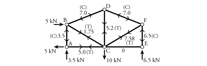   Figure 3.8: Method of Joints Example - Summary